ATCA Continuum Polarization Tutorial NGC612-CASA4.7
This CASA Guide is for Version 4.7 of CASA. If you are using a later version of CASA and this is the most recent available guide, then you should be able to use most, if not all, of this casaguide, as we try to limit script breaking changes in CASA development.
Overview
This CASA guide describes the calibration and imaging of a two-pointing continuum data set taken with the Australia Telescope Compact Array (ATCA) of the nearby radio galaxy NGC612. It has been adapted from the 3C391 Continuum Tutorial (CASA 4.6) for the VLA . The data were taken with 2048 MHz of bandwidth in 1 MHz channels, centered at 2.1 GHz, and recorded all polarizations. For ATCA data reduction there are two paths you can follow:
- If you are already familiar with the Miriad package, you can do the loading and optionally the flagging and calibration of the data in Miriad and then import the data into a CASA MeasurementSet with importmiriad.
- Alternatively, you can use importatca to load the ATCA archive files directly into CASA.
If this is your first attempt at using CASA for Compact Array data you are encouraged to start with a flagged and calibrated Miriad dataset and then try imaging the data. If you feel you are ready to tackle the full reduction job in CASA switch to the advanced guide
Obtaining the Data
For the purposes of this tutorial, we have created a starting data set, upon which several initial processing steps have already been conducted. You may obtain the data set from here(dataset size: 2.0GB).
The steps taken to produce this dataset were:
- The archive data was loaded into Miriad
- Basic data flagging of the calibration source was applied. These data were taken in the 1-3 GHz band, which has a lot of interference, especially in the lower part of the band.
- Bandpass, polarization leakage and fluxscale calibration was done using an observation of 1934-638
- Phase calibration was solved for on a secondary calibrator
- All the calibration was applied to the target source observations
- Further automated flagging was applied to the target
Once the download is complete, unzip and unpack the file (within a working directory in which you will then run CASA):
# In a Terminal:
tar xzvf ngc612.tgz
How to Use This CASA Guide
Here are a number of possible ways to run CASA, described in more detail in Getting Started in CASA. In brief, there are at least three different ways to run CASA:
- Interactively examining task inputs. In this mode, one types taskname to load the task, inp to examine the inputs, and go once those inputs have been set to your satisfaction. Allowed inputs are shown in blue and bad inputs are colored red. The input parameters themselves are changed one by one, e.g., selectdata=T. Screenshots of the inputs to various tasks used in the data reduction below are provided, to illustrate which parameters need to be set. More detailed help can be obtained on any task by typing help taskname. Once a task is run, the set of inputs are stored and can be retrieved via tget taskname; subsequent runs will overwrite the previous tget file.
- Pseudo-interactively via task function calls. In this case, all of the desired inputs to a task are provided at once on the CASA command line. This tutorial is made up of such calls, which were developed by looking at the inputs for each task and deciding what needed to be changed from default values. For task function calls, only parameters that you want to be different from their defaults need to be set.
- Non-interactively via a script. A series of task function calls can be combined together into a script, and run from within CASA via execfile('scriptname.py'). This and other CASA Tutorial Guides have been designed to be extracted into a script via the script extractor by using the method described at the Extracting_scripts_from_these_tutorials page. Should you use the script generated by the script extractor for this CASA Guide, be aware that it will require some small amount of interaction related to the plotting, occasionally suggesting that you close the graphics window and hitting return in the terminal to proceed. It is in fact unnecessary to close the graphics windows (it is suggested that you do so purely to keep your desktop uncluttered).
If you are a relative novice or just new to CASA, it is strongly recommended to work through this tutorial by cutting and pasting the task function calls provided below after you have read all the associated explanations. Work at your own pace, look at the inputs to the tasks to see what other options exist, and read the help files. Later, when you are more comfortable, you might try to extract the script, modify it for your purposes, and begin to reduce other data.
Importing the Miriad data
Before beginning our data reduction, we must start CASA. If you have not used CASA before, some helpful tips are available on the Getting Started in CASA page.
Once you have CASA up and running in the directory containing the data, then start your data reduction by getting the data into a MeasurementSet. The task to do this, importmiriad, is very simple. If your observation has a large range of system temperature you may want to use tsys=True to use the Tsys for the visibility weights, this will improve the noise level but may increase the sidelobe level in the synthesized beam.
# In CASA
importmiriad(mirfile='ngc612.uv',vis='ngc612.ms')
The Observation
Before diving into the imaging, lets have a look what we've got in our data. The task listobs can be used to get a listing of the individual scans comprising the observation, the frequency setup, source list, and antenna locations.
# In CASA
listobs(vis='ngc612.ms')
As you can see there are only two sources, called west_lobe and east_lobe. The galaxy ngc612 is quite large compared to the primary beam at 2 GHz, so two pointings were used to cover the emission with adequate sensitivity. The observation ran for close to 12 hours, this should give good uv coverage with the array in a short E-W configuration. From the antenna table we can see that antenna 1 to 5 are all within 750m and 6 is a long way off. We would generally not use antenna 6 for imaging in a 750m configuration unless we needed to get an accurate position for a point source or we were combining this observation with other configurations that fill in the large gap.
##########################################
##### Begin Task: listobs            #####
listobs(vis="ngc612.ms",selectdata=True,spw="",field="",antenna="",
        uvrange="",timerange="",correlation="",scan="",intent="",
        feed="",array="",observation="",verbose=True,listfile="",
        listunfl=False,cachesize=50,overwrite=False)
================================================================================
           MeasurementSet Name:  ngc612.ms      MS Version 2
================================================================================
   Observer: obs     Project: unknown
Observation: ATCA
Data records: 45115       Total elapsed time = 42269.9 seconds
   Observed from   25-Oct-2012/07:32:00.0   to   25-Oct-2012/19:16:29.9 (UTC)
Compute subscan properties

   ObservationID = 0         ArrayID = 0
  Date        Timerange (UTC)          Scan  FldId FieldName             nRows     SpwIds   Average Interval(s)    ScanIntent
  25-Oct-2012/07:32:00.0 - 07:40:49.9     0      0 east_lobe                  495  [0]  [9.86]
              07:41:10.0 - 07:46:09.9     1      1 west_lobe                  450  [0]  [9.86]
              07:46:30.0 - 07:51:29.9     2      0 east_lobe                  450  [0]  [9.86]
              07:52:00.0 - 07:56:59.9     3      1 west_lobe                  450  [0]  [9.86]
              07:57:20.0 - 08:02:19.9     4      0 east_lobe                  450  [0]  [9.86]
              08:02:40.0 - 08:07:49.9     5      1 west_lobe                  460  [0]  [9.86]
              08:08:10.0 - 08:13:09.9     6      0 east_lobe                  450  [0]  [9.86]
              08:13:30.0 - 08:18:29.9     7      1 west_lobe                  450  [0]  [9.86]
              08:18:50.0 - 08:23:49.9     8      0 east_lobe                  450  [0]  [9.86]
              08:24:10.0 - 08:29:09.9     9      1 west_lobe                  434  [0]  [9.86]
              08:34:50.0 - 08:39:49.9    10      0 east_lobe                  450  [0]  [9.86]
              08:40:10.0 - 08:45:09.9    11      1 west_lobe                  450  [0]  [9.86]
              09:23:00.0 - 09:27:59.9    12      0 east_lobe                  450  [0]  [9.86]
              09:28:20.0 - 09:33:19.9    13      1 west_lobe                  450  [0]  [9.86]
              09:33:40.0 - 09:38:39.9    14      0 east_lobe                  450  [0]  [9.86]
              09:39:00.0 - 09:43:59.9    15      1 west_lobe                  450  [0]  [9.86]
              09:44:20.0 - 09:49:19.9    16      0 east_lobe                  436  [0]  [9.86]
              09:49:40.0 - 09:54:39.9    17      1 west_lobe                  450  [0]  [9.86]
              09:55:00.0 - 09:59:59.9    18      0 east_lobe                  450  [0]  [9.86]
              10:00:20.0 - 10:05:19.9    19      1 west_lobe                  450  [0]  [9.86]
              10:05:40.0 - 10:10:39.9    20      0 east_lobe                  437  [0]  [9.86]
              10:11:00.0 - 10:15:59.9    21      1 west_lobe                  449  [0]  [9.86]
              10:21:40.0 - 10:26:39.9    22      0 east_lobe                  450  [0]  [9.86]
              10:27:00.0 - 10:31:59.9    23      1 west_lobe                  450  [0]  [9.86]
              10:32:20.0 - 10:37:19.9    24      0 east_lobe                  450  [0]  [9.86]
              10:37:40.0 - 10:42:39.9    25      1 west_lobe                  449  [0]  [9.86]
              10:43:00.0 - 10:47:59.9    26      0 east_lobe                  450  [0]  [9.86]
              10:48:20.0 - 10:53:19.9    27      1 west_lobe                  450  [0]  [9.86]
              10:53:40.0 - 10:58:39.9    28      0 east_lobe                  450  [0]  [9.86]
              10:59:00.0 - 11:03:59.9    29      1 west_lobe                  450  [0]  [9.86]
              11:04:20.0 - 11:09:19.9    30      0 east_lobe                  450  [0]  [9.86]
              11:09:40.0 - 11:14:39.9    31      1 west_lobe                  450  [0]  [9.86]
              11:20:40.0 - 11:25:39.9    32      0 east_lobe                  450  [0]  [9.86]
              11:26:00.0 - 11:30:59.9    33      1 west_lobe                  450  [0]  [9.86]
              11:31:20.0 - 11:36:19.9    34      0 east_lobe                  450  [0]  [9.86]
              11:36:40.0 - 11:41:39.9    35      1 west_lobe                  450  [0]  [9.86]
              11:42:00.0 - 11:46:59.9    36      0 east_lobe                  450  [0]  [9.86]
              11:47:20.0 - 11:52:19.9    37      1 west_lobe                  450  [0]  [9.86]
              12:19:50.0 - 12:24:49.9    38      0 east_lobe                  450  [0]  [9.86]
              12:25:10.0 - 12:30:09.9    39      1 west_lobe                  450  [0]  [9.86]
              12:30:30.0 - 12:35:29.9    40      0 east_lobe                  450  [0]  [9.86]
              12:35:50.0 - 12:40:49.9    41      1 west_lobe                  450  [0]  [9.86]
              12:41:10.0 - 12:46:09.9    42      0 east_lobe                  450  [0]  [9.86]
              12:46:30.0 - 12:51:29.9    43      1 west_lobe                  450  [0]  [9.86]
              12:51:50.0 - 12:56:49.9    44      0 east_lobe                  450  [0]  [9.86]
              12:57:10.0 - 13:02:09.9    45      1 west_lobe                  450  [0]  [9.86]
              13:02:30.0 - 13:07:29.9    46      0 east_lobe                  450  [0]  [9.86]
              13:07:50.0 - 13:12:49.9    47      1 west_lobe                  450  [0]  [9.86]
              13:19:30.0 - 13:24:29.9    48      0 east_lobe                  450  [0]  [9.86]
              13:24:50.0 - 13:29:49.9    49      1 west_lobe                  450  [0]  [9.86]
              13:30:10.0 - 13:35:09.9    50      0 east_lobe                  450  [0]  [9.86]
              13:35:30.0 - 13:40:29.9    51      1 west_lobe                  450  [0]  [9.86]
              13:40:50.0 - 13:45:49.9    52      0 east_lobe                  450  [0]  [9.86]
              13:46:10.0 - 13:51:09.9    53      1 west_lobe                  450  [0]  [9.86]
              13:51:30.0 - 13:56:29.9    54      0 east_lobe                  450  [0]  [9.86]
              13:56:50.0 - 14:01:49.9    55      1 west_lobe                  450  [0]  [9.86]
              14:02:10.0 - 14:07:09.9    56      0 east_lobe                  450  [0]  [9.86]
              14:07:30.0 - 14:12:29.9    57      1 west_lobe                  450  [0]  [9.86]
              14:18:10.0 - 14:23:09.9    58      0 east_lobe                  450  [0]  [9.86]
              14:23:30.0 - 14:28:29.9    59      1 west_lobe                  450  [0]  [9.86]
              14:28:50.0 - 14:33:49.9    60      0 east_lobe                  450  [0]  [9.86]
              14:34:10.0 - 14:39:09.9    61      1 west_lobe                  450  [0]  [9.86]
              14:39:30.0 - 14:44:29.9    62      0 east_lobe                  450  [0]  [9.86]
              14:44:50.0 - 14:49:49.9    63      1 west_lobe                  450  [0]  [9.86]
              15:20:50.0 - 15:25:49.9    64      0 east_lobe                  450  [0]  [9.86]
              15:26:10.0 - 15:31:09.9    65      1 west_lobe                  450  [0]  [9.86]
              15:31:30.0 - 15:36:29.9    66      0 east_lobe                  450  [0]  [9.86]
              15:36:50.0 - 15:41:49.9    67      1 west_lobe                  450  [0]  [9.86]
              15:42:10.0 - 15:47:09.9    68      0 east_lobe                  450  [0]  [9.86]
              15:47:30.0 - 15:52:29.9    69      1 west_lobe                  450  [0]  [9.86]
              15:52:50.0 - 15:57:49.9    70      0 east_lobe                  450  [0]  [9.86]
              15:58:10.0 - 16:03:09.9    71      1 west_lobe                  450  [0]  [9.86]
              16:03:30.0 - 16:08:29.9    72      0 east_lobe                  450  [0]  [9.86]
              16:08:50.0 - 16:13:49.9    73      1 west_lobe                  450  [0]  [9.86]
              16:19:30.0 - 16:24:29.9    74      0 east_lobe                  450  [0]  [9.86]
              16:24:50.0 - 16:29:49.9    75      1 west_lobe                  450  [0]  [9.86]
              16:30:10.0 - 16:35:09.9    76      0 east_lobe                  450  [0]  [9.86]
              16:35:30.0 - 16:40:29.9    77      1 west_lobe                  450  [0]  [9.86]
              16:40:50.0 - 16:45:49.9    78      0 east_lobe                  450  [0]  [9.86]
              16:46:10.0 - 16:51:09.9    79      1 west_lobe                  450  [0]  [9.86]
              16:51:30.0 - 16:56:29.9    80      0 east_lobe                  450  [0]  [9.86]
              16:56:50.0 - 17:01:49.9    81      1 west_lobe                  450  [0]  [9.86]
              17:02:10.0 - 17:07:09.9    82      0 east_lobe                  450  [0]  [9.86]
              17:07:30.0 - 17:12:29.9    83      1 west_lobe                  450  [0]  [9.86]
              17:17:50.0 - 17:22:49.9    84      0 east_lobe                  450  [0]  [9.86]
              17:23:10.0 - 17:28:09.9    85      1 west_lobe                  450  [0]  [9.86]
              17:28:30.0 - 17:33:29.9    86      0 east_lobe                  450  [0]  [9.86]
              17:33:50.0 - 17:38:49.9    87      1 west_lobe                  450  [0]  [9.86]
              17:39:10.0 - 17:44:09.9    88      0 east_lobe                  450  [0]  [9.86]
              17:44:30.0 - 17:49:29.9    89      1 west_lobe                  450  [0]  [9.86]
              18:17:00.0 - 18:21:59.9    90      0 east_lobe                  450  [0]  [9.86]
              18:22:20.0 - 18:27:19.9    91      1 west_lobe                  450  [0]  [9.86]
              18:27:40.0 - 18:32:39.9    92      0 east_lobe                  450  [0]  [9.86]
              18:33:00.0 - 18:37:59.9    93      1 west_lobe                  450  [0]  [9.86]
              18:38:20.0 - 18:43:19.9    94      0 east_lobe                  450  [0]  [9.86]
              18:43:40.0 - 18:48:39.9    95      1 west_lobe                  450  [0]  [9.86]
              18:49:00.0 - 18:53:59.9    96      0 east_lobe                  450  [0]  [9.86]
              18:54:20.0 - 18:59:19.9    97      1 west_lobe                  450  [0]  [9.86]
              18:59:40.0 - 19:04:39.9    98      0 east_lobe                  450  [0]  [9.86]
              19:05:00.0 - 19:09:59.9    99      1 west_lobe                  450  [0]  [9.86]
              19:15:20.0 - 19:16:29.9   100      0 east_lobe                  105  [0]  [9.86]
           (nRows = Total number of rows per scan)
Fields: 2
  ID   Code Name                RA               Decl           Epoch   SrcId      nRows
  0         east_lobe           01:34:16.760003 -36.30.13.52004 J2000   0          22623
  1         west_lobe           01:33:34.630993 -36.29.21.54998 J2000   1          22492
Spectral Windows:  (1 unique spectral windows and 1 unique polarization setups)
  SpwID  Name   #Chans   Frame   Ch0(MHz)  ChanWid(kHz)  TotBW(kHz) CtrFreq(MHz)  Corrs
  0              2049   TOPO    3124.000      1000.000   2048999.9   2099.9999   XX  XY  YX  YY
Sources: 2
  ID   Name                SpwId RestFreq(MHz)  SysVel(km/s)
  0    east_lobe           any   0              0
  1    west_lobe           any   0              0
Antennas: 6:
  ID   Name  Station   Diam.    Long.         Lat.                Offset from array center (m)                ITRF Geocentric coordinates (m)
                                                                     East         North     Elevation               x               y               z
  0    CA01  ANT1      22.0 m   +149.33.56.6  -30.08.43.7       1499.9964        0.7791       -1.6154 -4751674.968380  2791612.462760 -3200482.261996
  1    CA02  ANT2      22.0 m   +149.33.50.3  -30.08.43.7       1331.6268        0.6976       -1.7776 -4751589.522380  2791757.539760 -3200482.250996
  2    CA03  ANT3      22.0 m   +149.33.48.0  -30.08.43.7       1270.4080        0.6519       -1.8365 -4751558.446380  2791810.284760 -3200482.260996
  3    CA04  ANT4      22.0 m   +149.33.32.6  -30.08.43.7        857.1507        0.4408       -2.2258 -4751348.701380  2792166.358760 -3200482.247996
  4    CA05  ANT5      22.0 m   +149.33.28.0  -30.08.43.7        734.6981        0.3677       -2.3339 -4751286.547380  2792271.864760 -3200482.256996
  5    CA06  ANT6      22.0 m   +149.31.08.2  -30.08.43.8      -2999.9964       -0.8846       -4.6136 -4749390.961380  2795489.734760 -3200482.194996
##### End Task: listobs              #####
##########################################
Applying Parallactic Angle Calibration
The first thing we need to do when dealing with ATCA linear polarization data is correct for the parallactic angle rotation of the feeds with respect to the sky. Since the antennas have an Alt-Az mount and the receptors are linearly polarized, the X and Y receptors rotate on the sky. The calibration term 'P', for parallactic angle, corrects for this rotation. Without it the Stokes Q and U images will come out quite wrong. Since the 'P' calibration can be calculated exactly, all we need to do is run applycal with the parang parameter set to True.
# In CASA
applycal(vis='ngc612.ms',parang=True)
Multi-scale Polarization Clean

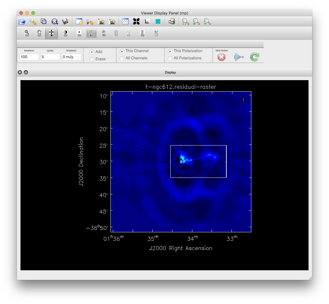
To image this data with 2 pointings we need to use mosaicing, and because the source is quite extended, we will also use the multiscale option. Because the lower part of the band has a lot of interference and the full 1.1-3.1 GHz band is too wide to image properly in one go (even with MFS) we will restrict the imaging for this tutorial to the top 1/3 of the band, which corresponds to the bottom 681 channels. (You could try imaging the rest of the band yourself.) To specify this selection we need to use 'spw='0:0~680', indicating channel 0 to 680 from spectral window 0. At an average frequency of about 2.7 GHz the primary beam is about 17' and the resolution for a 750m array is about 20" if we exclude CA06 (antenna='!5'). Based on this we'll choose a cell size of 5" and and image size of 500 pixels. We will make a test image to see what the field looks like and use the interactive option so we can set the area to clean. In the example we've used a simple box, but you can use polygons or other shapes. Once you have set the clean area you can save it to a file and then enter this as the mask for deeper cleaning later. After some experimentation we've chosen the multiscale parameter to correspond to: a point source, about twice the beam and about the size of the largest 'blob' in the image. Setting the largest scale much smaller tends to leave a negative bowl around the source.
# In CASA
clean(vis='ngc612.ms',imagename='t-ngc612',spw='0:0~680',imagermode='mosaic',multiscale=[0,8,24],
          imsize=500,cell='5.0arcsec',stokes='I',weighting='briggs',robust=0.5,antenna='!5',interactive=True)

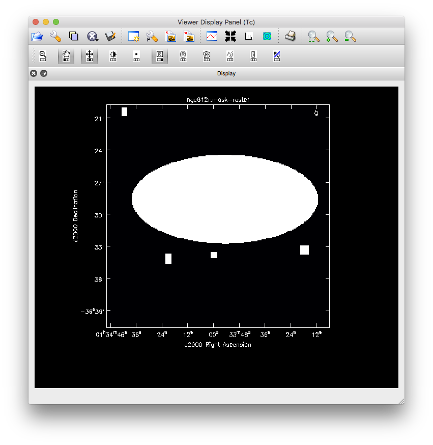
Now that we have a feel for what the source looks like, we can clean a bit deeper and do all the Stokes parameters. A few point sources outside the central area appear with this deeper clean, so we should really redo the clean with those sources added into the mask. Figure 3 shows the mask used in the final clean: using the viewer region editor we changed the box to an ellipse and added 4 boxes around point sources. You can get the region file here: Media:ngc612region.txt, after you download it, rename it to ngc612region.crtf.

# In CASA
clean(vis='ngc612.ms',imagename='ngc612h',spw='0:0~680',imagermode='mosaic',multiscale=[0,8,24],
          imsize=500,cell='5.0arcsec',stokes='IQUV',weighting='briggs',robust=0.5,niter=10000,threshold='0.5mJy',
          antenna='!5',mask='ngc612region.crtf' )
Constructing Polarization Intensity and Angle Images
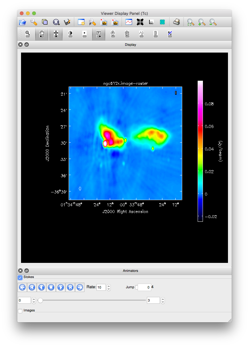
We've made a full polarization image of ngc612. This image is actually a cube with the standard two angular dimensions (right ascension, declination) and a third dimension containing the polarization information. Considering the image cube as a matrix, [math]\displaystyle{ Image[l,m,p] }[/math], the [math]\displaystyle{ l }[/math] and [math]\displaystyle{ m }[/math] axis describe the sky brightness or intensity for the given [math]\displaystyle{ p }[/math] axis. If one opens the viewer and loads the ngc612 continuum image, the default view contains an animator or pane with movie controls. One can step through the polarization axis, displaying the images for the different polarizations.
As created, the image contains four polarizations, one for each of the four Stokes parameters: I, Q, U, and V. Recall that Stokes Q and U describe linear polarization and V describes circular polarization. Specifically, Q describes the amount of linear polarization aligned with a given axis, and U describes the amount of linear polarization at a 45 deg angle to that axis. The V parameter describes the amount of circular polarization, with the sign (positive or negative) describing the sense of the circular polarization (right- or left-hand circularly polarized).
Few celestial sources, with the notable exception of masers, are expected to show circular polarization. Terrestrial and satellite sources, however, are often highly circularly polarized. The V image is therefore often worth forming because any V emission could be indicative of unflagged RFI within the data (or problems with the calibration!). In our image we can see some remnant Stokes V at the position of the strongest source and an error pattern around it that has not cleaned away. This indicates it is probably due to remaining calibration errors.
Because the Q and U images both describe the amount of linear polarization, it is more common to work with a linear polarization intensity image, [math]\displaystyle{ P = \sqrt{Q^2 +U^2} }[/math] and the polarization position angle [math]\displaystyle{ tan 2\chi = U/Q }[/math].
1. Combine the Q and U images using the parameter mode='poli' of immath to form the linear polarization image. Because P is formed from the sum of the squares of the Q and U values, it is biased by the noise. You can set the sigma value to debias this (it subtracts the square of this value from the Q2+U2 before taking the square-root). Use the imstat task to get the rms in Stokes V, which will usually give a good estimate of the noise. You could just look at the output and enter the rms value as sigma in immath, adding the correct units. Here we show how to do this from a script by capturing the output of imstat into a variable and then extracting the rms value; because the returned value is an array we need to index it with 0 to get the value as a floating point number: s['rms'][0]. Because immath's sigma parameter expects a string value, we convert the float value into a string with a '%f' format.
# In CASA
s=imstat(imagename='ngc612h.image',stokes='V')
sigma='%f Jy/beam' % s['rms'][0]
immath(imagename='ngc612h.image',mode='poli',outfile='ngc612h.P',sigma=sigma)
You'll notice that immath is smart enough to extract the Q and U planes out of our cube into temporary images and use them to create the 'P' image.
2. Combine the Q and U images using the parameter mode='pola' of immath to form the polarization position angle image. To avoid displaying the position angle of noise, we can set a threshold intensity of the linear polarization, above which we wish to calculate the polarization angle, using the parameter polithresh. An appropriate level here might be the [math]\displaystyle{ 5\sigma }[/math] level of around 1 mJy/beam:

# In CASA
immath(imagename='ngc612h.image',mode='pola',outfile='ngc612h.X',polithresh='1mJy/beam')
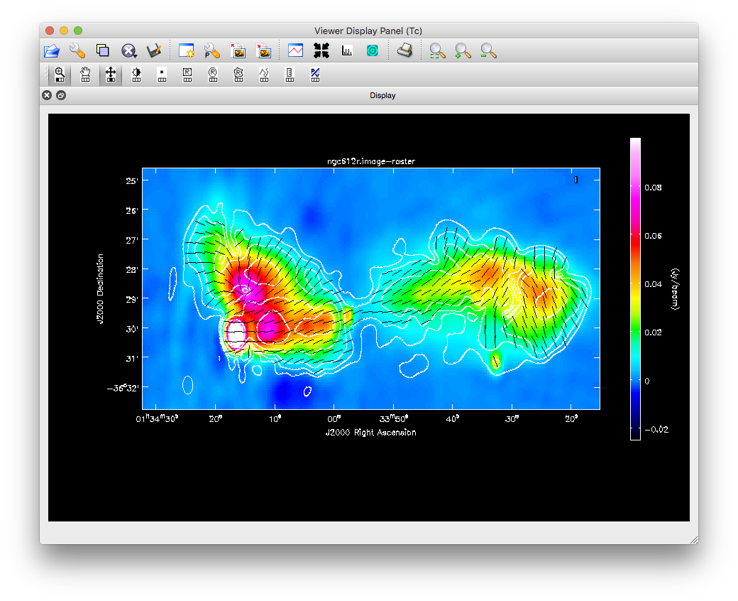
3. Now use the viewer to display all the images together:
- load the cube as a raster image and set the levels so you can see the extended emission
- load the linear polarization image as a contour image, set the contours to 200,100,50,20,10 and 5 times the noise level of 0.2 mJy/beam
- load the polarization image as a vector image, you can switch the line color to black to make it stand out more
The result should look something like Figure 4.
4. We'll extract some statistics so you can compare them with your own results:
- The total polarized flux in the lobes above the 2 mJy contour.
- The change in average polarization angle across the western lobe.
# In CASA
mystats1=imstat(imagename='ngc612h.P',mask='ngc612h.P>0.002')
mystats2=imstat(imagename='ngc612h.X',region='box [ [ 325pix , 260pix] , [345pix, 275pix ] ]')
mystats3=imstat(imagename='ngc612h.X',region='box [ [ 365pix , 250pix] , [385pix,  265pix ] ]')

print 'Total polarized flux density: %6.3f Jy' % mystats1['flux']
print 'Pol. angles in western lobe: %4.1f and %4.1f degrees' % (mystats2['mean'],mystats3['mean'])
Running the above commands should produce something close to the following output:
Total polarized flux density: 1.166 Jy
Pol. angles in western lobe: -61.7 and 22.8 degrees
5. As further practice you could try to image the rest of the band by changing the channel selection and imaging the middle and lower part of the band. You may need to do some additional flagging to get a decent image.
Questions about this tutorial? Please contact the NRAO Helpdesk.
Last checked on CASA Version 5.6.2.