M100 Band3 SingleDish 5.1
- This guide requires CASA 5.1.0 and assumes that you have downloaded M100_Band3_TP_UncalibratedData.tgz as described in M100_Band3#Obtaining_the_Data
- The processes described below WILL NOT OPERATE in CASA versions earlier than 5.1.0
- A previous version of this guide can be found at M100_Band3_SingleDish_4.5
- Details of the ALMA observations are described at M100_Band3
- This portion of the guide covers calibration and imaging starting from the raw visibility data.
Overview
This portion of CASA Guide will cover the data reduction of the Total Power (TP) array observations of M100. The objective is to generate from the TP dataset, a position-position-velocity cube suitable for merging with 7m and 12m datasets.
The data consist of "amplitude calibrator" datasets (containing observational data of the quasar 3C279) and "science" datasets containing data for the science target M100. To be clear - the observations of 3C279 and M100 both follow the same general process - i.e. they are themselves calibrated with frequent observations of blank sky - the so-called 'OFF', which is used to determine the System temperature as a function of frequency, and form a referenced bandpass, in units of Antenna Temperature (Ta*) [K].
Ultimately the quasar data are compared with recent flux measurements (in Jy/beam), obtained from archived 12m data, to determine the scaling factor between Ta* and Jy/beam, and that scaling factor is then applied to the science data, to bootstrap to Jy/beam.
The combination of the resultant image with the interferometric (12-m array and 7-m array) data is explained in a separate page, valid for CASA versions 4.3 and later M100_Band3_Combine_4.3.
This guide is designed for CASA 5.1.0.
Confirm Your Version of CASA
This guide has been written for CASA release 5.1.0. Please confirm your version before proceeding. The value returned from cu.version_string() should be 5.1.0. If not, please obtain at least version 5.1.0 (or later), from [1]
# In CASA
version = cu.version_string()
print "You are using " + version
if (version < '5.1.0'):
    print "YOUR VERSION OF CASA IS TOO OLD FOR THIS GUIDE."
    print "PLEASE UPDATE IT BEFORE PROCEEDING."
else:
    print "Your version of CASA is appropriate for this guide."
Summary of Datasets
The observations were made on the 1st, 5th, 7th, and 17th July 2014, using two or three 12-m antennas and the ACA correlator. The table below indicates the ID's of the Execution Blocks, their start and end times, and the antennas in the array. There are nine science datasets (i.e., two or three per day).
#Science
uid___A002_X85c183_X36f      Observed from 2014-07-01T21:51:26.2 to 2014-07-01T22:40:28.4 (UTC)      DA61, PM03, PM04
uid___A002_X85c183_X60b      Observed from 2014-07-01T22:43:50.0 to 2014-07-01T23:32:39.6 (UTC)      DA61, PM03, PM04
uid___A002_X8602fa_X2ab      Observed from 2014-07-05T23:58:03.6 to 2014-07-06T00:46:52.0 (UTC)      PM02, PM03, PM04
uid___A002_X8602fa_X577      Observed from 2014-07-06T00:55:17.8 to 2014-07-06T01:44:07.3 (UTC)      PM02, PM03, PM04
uid___A002_X864236_X2d4      Observed from 2014-07-07T23:03:48.1 to 2014-07-07T23:53:47.9 (UTC)      PM03, PM04
uid___A002_X864236_X693      Observed from 2014-07-07T23:56:09.6 to 2014-07-08T00:46:07.1 (UTC)      PM03, PM04
uid___A002_X86fcfa_Xd9       Observed from 2014-07-17T20:55:15.5 to 2014-07-17T21:44:06.1 (UTC)      DV10, PM03, PM04
uid___A002_X86fcfa_X664      Observed from 2014-07-17T22:24:17.3 to 2014-07-17T23:13:08.0 (UTC)      DV10, PM03, PM04
uid___A002_X86fcfa_X96c      Observed from 2014-07-17T23:23:37.0 to 2014-07-18T00:12:25.3 (UTC)      DV10, PM03, PM04
Similarly, the concomitant Calibration datasets (used to convert from Antenna temperature units into Jy/beam units, for combination), are:
#Amplitude Calibrator
uid___A002_X85c183_X895      Observed from 2014-07-01T23:35:23.1 to 2014-07-02T00:07:54.6 (UTC)      DA61, PM03, PM04
uid___A002_X8602fa_Xc3       Observed from 2014-07-05T23:21:25.6 to 2014-07-05T23:53:41.0 (UTC)      PM02, PM03, PM04
uid___A002_X864236_Xe1       Observed from 2014-07-07T22:27:35.4 to 2014-07-07T23:01:05.7 (UTC)      PM03, PM04
uid___A002_X86fcfa_X3ae      Observed from 2014-07-17T21:48:30.0 to 2014-07-17T22:20:52.2 (UTC)      DV10, PM03, PM04
Script Calibration
The scripts listed below process all the single-dish science and calibrator data, using a few loops.
- (optional) The calibrator (i.e. quasar) data are processed (see the section, 'Imaging the Amplitude Calibrator and Measure the Value of Jy/K' in below)
- The science data are processed with - M100.casa5p1.calib.py
- and the (calibrated) science data are imaged with - M100.casa5p1.imaging.py
Executing each of these scripts in order, will be sufficient to calibrate and image the science data (although the calibrator processing script can be omitted, as the relevant parameters are actually already explicitly written into the script).
They can be invoked from the command line using the execfile command.
# In CASA
execfile('M100.casa5p1.calib.py')
Manual Calibration
By way of description, and as a means to introduce and demonstrate some of the interactive and diagnostic tools here we describe in more detail, the steps taken by the scripts - although in this case we demonstrate the process for only one of the ASDM datasets. In the Imaging section, we assume all the ASDMs are appropriately reduced either by the manual process, or by using the script.
The entire process takes less than 30 minutes.
There are three basic steps to the Calibration of the Science data:
- Import, inspection and flagging
- Calibration
- Sky and bandpass calibration (i.e. Tsys and frequency sampling function)
- Adjustment for Correlator non-linearity (this step is necessary only for data taken in ALMA Cycle 3 and earlier)
- Conversion to Jy/beam
- Imaging
Import "Analysis Utilities"
The Analysis_Utilities package will be used most critically for the imaging processes. While it is not necessary for completing the calibration stages, it is used to check data quality, and should be loaded.
Import the package from https://casaguides.nrao.edu/index.php/Analysis_Utilities, and apply the class therein.
# In CASA
import analysisUtils as aU
Import, inspection and flagging
Import
The first thing to do is to convert the dataset into the CASA Measurement Set (MS) format. The raw data have been provided to you in the ASDM (ALMA Science Data Model), which is the native format of the data produced by the observatory but cannot be processed by CASA. The conversion from ASDM to MS is done with the task importasdm.
# In CASA
importasdm('uid___A002_X85c183_X36f',
           asis='Antenna Station Receiver Source CalAtmosphere CalWVR', bdfflags=False)
os.system(os.environ['CASAPATH'].split()[0] + '/bin/bdflags2MS -f "COR DELA INT MIS SIG SYN TFB WVR ZER" uid___A002_X85c183_X36f uid___A002_X85c183_X36f.ms')
The converted dataset (with a suffix ".ms") is created and then flags embedded in the ASDM dataset (so-called "BDF flags") are transferred to MS using the command bdflags2MS.
Note: The above code should be used for cycle 2 data, or earlier. Cycle 3+ data can simply use:
# In CASA
importasdm('uid___A002_X85c183_X36f',
           asis='Antenna Station Receiver Source CalAtmosphere CalWVR', bdfflags=True)
Inspection - listobs
After import, the usual first step is then to get some basic information about the data. We do this using the task listobs, which will output a detailed summary of each dataset supplied.
# In CASA
listobs(vis='uid___A002_X85c183_X36f.ms',
        listfile='uid___A002_X85c183_X36f.ms.listobs')
The output will be written in a file named uid___A002_X85c183_X36f.ms.listobs which you can (and should) view at your leisure. listobs displays information about the targets, dates, frequencies, etc. Below is an excerpt from listobs for uid___A002_X85c183_X36f:
Fields: 2
  ID   Code Name                RA               Decl           Epoch   SrcId      nRows
  0    none J1215+1654          12:15:03.979140 +16.54.37.95680 J2000   0          14661
  1    none M100                12:22:54.360000 +15.48.50.60000 J2000   1          61653
Spectral Windows:  (25 unique spectral windows and 2 unique polarization setups)
  SpwID  Name                           #Chans   Frame   Ch0(MHz)  ChanWid(kHz)  TotBW(kHz) CtrFreq(MHz) BBC Num  Corrs
  0      WVR#NOMINAL                         4   TOPO  184550.000   1500000.000   7500000.0 187550.0000        0  XX
  1      ALMA_RB_03#BB_1#SW-01#FULL_RES    124   TOPO   91955.512    -15625.000   1937500.0  90994.5750        1  XX  YY
  2      ALMA_RB_03#BB_1#SW-01#CH_AVG        1   TOPO   90978.950   1734375.000   1734375.0  90978.9500        1  XX  YY
  3      ALMA_RB_03#BB_2#SW-01#FULL_RES    124   TOPO   93893.012    -15625.000   1937500.0  92932.0750        2  XX  YY
  4      ALMA_RB_03#BB_2#SW-01#CH_AVG        1   TOPO   92924.262   1937500.000   1937500.0  92924.2625        2  XX  YY
  5      ALMA_RB_03#BB_3#SW-01#FULL_RES    124   TOPO  102033.637     15625.000   1937500.0 102994.5750        3  XX  YY
  6      ALMA_RB_03#BB_3#SW-01#CH_AVG        1   TOPO  102986.762   1937500.000   1937500.0 102986.7625        3  XX  YY
  7      ALMA_RB_03#BB_4#SW-01#FULL_RES    124   TOPO  104033.637     15625.000   1937500.0 104994.5750        4  XX  YY
  8      ALMA_RB_03#BB_4#SW-01#CH_AVG        1   TOPO  104986.762   1937500.000   1937500.0 104986.7625        4  XX  YY
  9      ALMA_RB_03#BB_1#SW-01#FULL_RES    128   TOPO  101942.187    -15625.000   2000000.0 100950.0000        1  XX  YY
  10     ALMA_RB_03#BB_1#SW-01#CH_AVG        1   TOPO  100926.562   1781250.000   1781250.0 100926.5625        1  XX  YY
  11     ALMA_RB_03#BB_2#SW-01#FULL_RES    128   TOPO  103757.337    -15625.000   2000000.0 102765.1500        2  XX  YY
  12     ALMA_RB_03#BB_2#SW-01#CH_AVG        1   TOPO  102741.712   1781250.000   1781250.0 102741.7125        2  XX  YY
  13     ALMA_RB_03#BB_3#SW-01#FULL_RES    128   TOPO  111814.962     15625.000   2000000.0 112807.1500        3  XX  YY
  14     ALMA_RB_03#BB_3#SW-01#CH_AVG        1   TOPO  112783.712   1781250.000   1781250.0 112783.7125        3  XX  YY
  15     ALMA_RB_03#BB_4#SW-01#FULL_RES    128   TOPO  113689.962     15625.000   2000000.0 114682.1500        4  XX  YY
  16     ALMA_RB_03#BB_4#SW-01#CH_AVG        1   TOPO  114658.712   1781250.000   1781250.0 114658.7125        4  XX  YY
  17     ALMA_RB_03#BB_1#SW-01#FULL_RES   4080   TOPO  101945.850      -488.281   1992187.5 100950.0000        1  XX  YY
  18     ALMA_RB_03#BB_1#SW-01#CH_AVG        1   TOPO  100949.756   1992187.500   1992187.5 100949.7559        1  XX  YY
  19     ALMA_RB_03#BB_2#SW-01#FULL_RES   4080   TOPO  103761.000      -488.281   1992187.5 102765.1500        2  XX  YY
  20     ALMA_RB_03#BB_2#SW-01#CH_AVG        1   TOPO  102764.906   1992187.500   1992187.5 102764.9059        2  XX  YY
  21     ALMA_RB_03#BB_3#SW-01#FULL_RES   4080   TOPO  111811.300       488.281   1992187.5 112807.1500        3  XX  YY
  22     ALMA_RB_03#BB_3#SW-01#CH_AVG        1   TOPO  112806.906   1992187.500   1992187.5 112806.9059        3  XX  YY
  23     ALMA_RB_03#BB_4#SW-01#FULL_RES   4080   TOPO  113686.300       488.281   1992187.5 114682.1500        4  XX  YY
  24     ALMA_RB_03#BB_4#SW-01#CH_AVG        1   TOPO  114681.906   1992187.500   1992187.5 114681.9059        4  XX  YY
Sources: 48
  ID   Name                SpwId RestFreq(MHz)  SysVel(km/s)
  0    J1215+1654          0     -              -
  0    J1215+1654          25    -              -
  0    J1215+1654          26    -              -
  0    J1215+1654          27    -              -
  0    J1215+1654          1     -              -
  0    J1215+1654          2     -              -
  0    J1215+1654          3     -              -
  0    J1215+1654          4     -              -
  0    J1215+1654          5     -              -
  0    J1215+1654          6     -              -
  0    J1215+1654          7     -              -
  0    J1215+1654          8     -              -
  0    J1215+1654          9     -              -
  0    J1215+1654          10    -              -
  0    J1215+1654          11    -              -
  0    J1215+1654          12    -              -
  0    J1215+1654          13    -              -
  0    J1215+1654          14    -              -
  0    J1215+1654          15    -              -
  0    J1215+1654          16    -              -
  0    J1215+1654          17    100950         0
  0    J1215+1654          18    100950         0
  0    J1215+1654          19    102794.1       0
  0    J1215+1654          20    102794.1       0
  0    J1215+1654          21    112794.1       0
  0    J1215+1654          22    112794.1       0
  0    J1215+1654          23    114669.1       0
  0    J1215+1654          24    114669.1       0
  1    M100                0     -              -
  1    M100                25    -              -
  1    M100                26    -              -
  1    M100                27    -              -
  1    M100                9     -              -
  1    M100                10    -              -
  1    M100                11    -              -
  1    M100                12    -              -
  1    M100                13    -              -
  1    M100                14    -              -
  1    M100                15    -              -
  1    M100                16    -              -
  1    M100                17    100950         0
  1    M100                18    100950         0
  1    M100                19    102794.1       0
  1    M100                20    102794.1       0
  1    M100                21    112794.1       0
  1    M100                22    112794.1       0
  1    M100                23    114669.1       0
  1    M100                24    114669.1       0
Antennas: 3:
  ID   Name  Station   Diam.    Long.         Lat.                Offset from array center (m)                ITRF Geocentric coordinates (m)
                                                                     East         North     Elevation               x               y               z
  0    DA61  A075      12.0 m   -067.45.17.9  -22.53.21.4         -4.5609     -499.7012       23.0322  2225072.419944 -5440148.858968 -2481499.171703
  1    PM03  T701      12.0 m   -067.45.18.8  -22.53.22.2        -29.1265     -522.7875       22.2052  2225045.995589 -5440149.141967 -2481520.118569
  2    PM04  T703      12.0 m   -067.45.16.2  -22.53.23.9         42.8797     -575.6910       21.7763  2225104.700870 -5440102.471978 -2481568.689518
From this output you can for example see the followings.
- From "Data records" section (not shown here): The execution consists of 15 scans with various scan intents.
- Scans 1 and 2 are pointing and sideband gain ratio calibrations (done interferometrically), which need to be done prior to observing the target, on the quasar J1215+1654.
- Scans 3 and 4 are interferometric delay and system noise temperature (Tsys) measurements also on J1215+1654 (they are in principle unnecessary; just a hack to make things happen on the telescope control software).
- Scans 6, 7, 9, 10, 12, 13, and 15, whose scan intents contain "OBSERVE_TARGET", are for raster mapping of the target M100. The associated spectral window (SPW) ID's are 0 and 17-24.
- Scans 5, 8, 11, and 14 with scan intents "CALIBRATE_ATMOSPHERE" are Tsys measurements for M100. The SPW ID's for Tsys scans are 0 and 9-16.
- From "Spectral Windows" section:
- SPW 0 contains the Water Vapor Radiometer (WVR) data, which are taken for all scans, but which are not used here.
- SPW's 1, 3, 5, and 7 are placed on standard continuum frequencies and are used for the pointing scan only.
- SPW's 9, 11, 13, and 15 cover the same frequency range as the science SPW's (see the next bullet) and are used to measure the Tsys used for calibration. They have 128 spectral channels (15.6 MHz spacing) in 2000 MHz bandwidth.
- SPW's 17, 19, 21, and 23 cover the frequency ranges used for the actual science observations. They have 4080 spectral channels (488 kHz spacing) in 1992 MHz bandwidth. Hereafter these SPW's are referred to as "science" SPW's. The target line, CO J=1-0, is placed in SPW 23, the corresponding Tsys is taken from SPW 15.
- The remaining, even-number SPW's contain channel-averages of the actually used SPW's (e.g., SPW 24 corresponds to SPW 23 averaged into one channel).
- From "Antennas" section: Three 12-m antennas (DA61, PM03, and PM04) were used for the observations.
Inspection - scanpattern
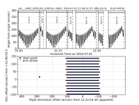
The scan pattern of the raster mapping can be visualized by issuing the following command (after import of Analysis Utils - see the top of this page for information). A plot will be shown in a window and also saved as a PNG file uid___A002_X85c183_X36f.ms.sampling.png.
# In CASA
aU.getTPSampling(vis='uid___A002_X85c183_X36f.ms',
                 showplot=True,
                 plotfile='uid___A002_X85c183_X36f.ms.sampling.png')
Inspection - System Noise Temperature
Let's start by checking the Tsys. We use the task gencal to extract the Tsys into a CASA calibration table. This table is only used for inspection of Tsys quality, and not in further processing.
# In CASA
gencal(vis='uid___A002_X85c183_X36f.ms',
       caltable='uid___A002_X85c183_X36f.ms.tsys',
       caltype='tsys')
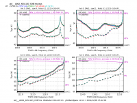
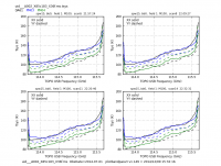
The generated Tsys calibration table can be plotted using the task plotbandpass. The generated plots are saved in the directories uid___A002_X85c183_X36f.ms.tsys.plots.overlayTime and uid___A002_X85c183_X36f.ms.tsys.plots.
# In CASA
plotbandpass(caltable='uid___A002_X85c183_X36f.ms.tsys',
             overlay='time',
             xaxis='freq',
             yaxis='amp',
             subplot=22,
             buildpdf=False,
             interactive=False,
             showatm=True,
             pwv='auto',
             chanrange='5~123',
             showfdm=True,
             field='',
             figfile='uid___A002_X85c183_X36f.ms.tsys.plots.overlayTime/uid___A002_X85c183_X36f.ms.tsys')
Flagging
Although the "science" SPW's have 1992 MHz bandwidths with 4080 spectral channels, their edge channels can be very noisy because each intermediate frequency signal path (baseband) is equipped with a bandpass filter of ~1.8 GHz width. Note that this is not necessarily always the case, it is in general, safest to flag out the edge channels, unless a spectral line of interest falls very close to the edge of the SPW band-edge. We flag 120 channels on each side of the "science" SPW's.
# In CASA
flagdata(vis = 'uid___A002_X85c183_X36f.ms',
       mode = 'manual',
       spw = '17:0~119;3960~4079,19:0~119;3960~4079,21:0~119;3960~4079,23:0~119;3960~4079',
       action = 'apply',
       flagbackup = True)
Calibration - sky, bandpass, nonlinearity and baseline
Tsys Calibration
We calibrate the data into Antenna temperature in units of K, using the equation Ta* = Tsys*(ON-OFF)/OFF, where ON and OFF are the data on-source (i.e., during the raster scanning) and off-source (on a reference position where only background emission exists), respectively. The calibration is done by the task sdcal which requires matching of list of the "science" and Tsys spectral windows. Tsys observations will always have 128 channels over 2GHz bandwidth, and as described in listobs, we already know which spectral windows match the science spectral windows most closely, in frequency. for example, spectral window 9, with 128 channels matches well with spectral window 17, 11 with 19, 13 with 21 and 15 with 2. Thus, we form the Tsys and Science spectral window mapping input parameters, with the syntax: {9:[17], 11:[19], 13:[21],15:[23]}
  9      ALMA_RB_03#BB_1#SW-01#FULL_RES    128   TOPO  101942.187    -15625.000   2000000.0 100950.0000        1  XX  YY
  .
  .
  17     ALMA_RB_03#BB_1#SW-01#FULL_RES   4080   TOPO  101945.850      -488.281   1992187.5 100950.0000        1  XX  YY
  11     ALMA_RB_03#BB_2#SW-01#FULL_RES    128   TOPO  103757.337    -15625.000   2000000.0 102765.1500        2  XX  YY
  .
  .
  19     ALMA_RB_03#BB_2#SW-01#FULL_RES   4080   TOPO  103761.000      -488.281   1992187.5 102765.1500        2  XX  YY
  13     ALMA_RB_03#BB_3#SW-01#FULL_RES    128   TOPO  111814.962     15625.000   2000000.0 112807.1500        3  XX  YY
  .
  .
  21     ALMA_RB_03#BB_3#SW-01#FULL_RES   4080   TOPO  111811.300       488.281   1992187.5 112807.1500        3  XX  YY
  15     ALMA_RB_03#BB_4#SW-01#FULL_RES    128   TOPO  113689.962     15625.000   2000000.0 114682.1500        4  XX  YY
  .
  .
  23     ALMA_RB_03#BB_4#SW-01#FULL_RES   4080   TOPO  113686.300       488.281   1992187.5 114682.1500        4  XX  YY
And the Tsys calibration command is formed like the following:
# In CASA
sdcal(infile = 'uid___A002_X85c183_X36f.ms',
    calmode = 'ps,tsys,apply',
    spwmap = {9:[17], 11:[19], 13:[21],15:[23]},
    spw = '17,19,21,23')
Note: in this step, the calibrations are applied in situ. That is: the calibrated data are written into the original data - however it is written in such a way that any additional calls to sdcal will not apply any further calibrations. We will examine the quality of the bandpass and Tsys calibration after the correction for non-linearity, next.
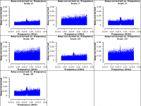
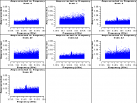
The calibrated bandpasses, averaged over each scan, can be plotted with:
# In CASA
plotms(vis='uid___A002_X85c183_X36f.ms',
    xaxis='freq', yaxis='amp', ydatacolumn='corrected',
    field='M100',spw='23',
    scan='6,7,9,10,12,13,15',
    averagedata=True,avgtime='9999',
    gridcols=3,gridrows=3,iteraxis='scan',
    plotrange=[113.5, 116, -0.01, 0.08],
    plotfile='vis.png',
    showgui=False)
Note: For amplitude calibrator datasets, (as opposed to science target maps) the calmode option for sdcal should be 'otfraster,tsys,apply' ('otfraster' instead of 'ps'). 'otfraster' tells the task to use both ends of each raster row as "OFF" data (as opposed to a dedicated "OFF" sky measurement). This is because temporal fluctuation of atmospheric emission is the dominant source of noise in radio continuum observations, and hence the "OFF" needs to be as close as possible to the "ON" in time (and spatial location).
Application of Non-Linearity Correction Factor
In Cycle 1 and 2, single-dish data taken with the ACA correlator suffer from non-linearity which originates in the digital signal processing. Its impact was thoroughly studied both experimentally and theoretically, and it was concluded that multiplication by a correction factor of 1.25 yields an amplitude accuracy of +/-5%.
To preserve the data history, we use here the tasks split to split out the science corrected data columns - note that from here on, the spectral windows are renumbered: [0,1,2,3]. We then generate a calibration table, using a defined function to_amp_factor, with gencal. Finally, we apply the calibration with applycal. We apply the correction here using tasks gencal and applycal - this is different to the methods used in the past, and are available now because of the migration to MS-only format of Single-dish CASA.
Note: The ACA online software has been equipped with this correction for data from cycle 3 and later (it should be applied for data from cycle 2 and earlier).
# In CASA
to_amp_factor = lambda x: 1. / sqrt(x)

split(vis='uid___A002_X85c183_X36f.ms',
    outputvis='uid___A002_X85c183_X36f.ms.cal.split',
    datacolumn='corrected',
    spw='17,19,21,23')

gencal(vis='uid___A002_X85c183_X36f.ms.cal.split',
    caltable='uid___A002_X85c183_X36f.ms.nlc',
    caltype='amp', spw='',
    parameter=[to_amp_factor(1.25)])

applycal(vis='uid___A002_X85c183_X36f.ms.cal.split',
    gaintable='uid___A002_X85c183_X36f.ms.nlc')
Note: the Python command lambda simply defines a function. Thus the line above : to_amp_factor = lambda x: 1. / sqrt(x) defines a function where the call: to_amp_factor(4) will return: 0.5
Baseline Subtraction (only for Science Datasets)
Note: this step is appropriate for spectral line observations (science datasets) but should not be done for the continuum observations (amplitude calibrator datasets) -- it would eliminate the continuum emission! Note: this step is optional and need not be completed to produce an image - however it is recommended for the majority of cases (esp. where the bandpass is affected by low-order modulations, and where the line-emission does not completely dominate the bandpass.)
We will subtract low-order spectral baselines using the task sdbaseline. Typically these manifest from structure in the distribution of water in the atmosphere: the ON and OFF positions are slightly different, and the difference manifests as - typically - a low frequency variation in the spectra. The situation is exacerbated for observations closer to water lines and also for higher frequencies.
# In CASA
sdbaseline(infile='uid___A002_X85c183_X36f.ms.cal.split',
    datacolumn='corrected',
     spw='',
     blfunc='poly',
     order=1,
     outfile='uid___A002_X85c183_X36f.ms.bl',
     overwrite=True)
The spectra can be checked using plotms, which we have already used in a previous step.
# In CASA
plotms(vis='uid___A002_X85c183_X36f.ms.bl',
    xaxis='freq', yaxis='amp', ydatacolumn='corrected',
    field='M100',spw='3',
    scan='6,7,9,10,12,13,15',
    averagedata=True,avgtime='9999',
    gridcols=3,gridrows=3,iteraxis='scan',
    plotrange=[113.5, 116, -0.01, 0.08],
    plotfile='vis_bl.png',
    showgui=False)
We do not concatenate separate Execution Blocks, because we need to determine and apply day-by-day Jy/K conversion factor.
Note that one of the antennas, PM02, had a problem in the first baseband (SPW 17) on 2014-07-05, and its impact may not be specific to this one SPW (e.g., it may have resulted in poor pointing calibration). Therefore the PM02 data should be flagged from the affected datasets: uid___A002_X8602fa_X2ab (science), and uid___A002_X8602fa_X577 (science). The calibrator set uid___A002_X8602fa_Xc3 will also be affected, and will be flagged out in the subsequent processing of the calibrators.
# In CASA
flagdata(vis='uid___A002_X8602fa_X2ab.ms.bl',
    antenna='PM02&&&')
flagdata(vis='uid___A002_X8602fa_X577.ms.bl',
    antenna='PM02&&&')
Convert science data from Kelvin to Jansky
At this stage the data have been calibrated into units of antenna temperature, in Kelvins.
It now remains to convert the science data into Jy/beam units - the Jy per K factors. This is important for combination of the data, with 7m and 12m sets. Later in this guide we show how to determine the correct factors from the calibrator datasets, for conversion (the process is essentially identical to processing the science datasets, with the exception that the baseline step is omitted from the calibration dataset processing). However to determine the factors, the calibration data must also be imaged and then interrogated to determine the appropriate values.
Applying the calibration factors to the science data is the last step in the script M100.casa5p1.calib.py.
We continue to use only one ASDM as an example; uid___A002_X85c183_X36f. The script should be consulted for treatment of all the M100 Single-dish ASDMs (and the correct application of the Jy per K factors). Again, we apply the factors by making use of the gencal and applycal tasks. Also as before, we make use of the python function defined earlier: to_amp_factor
# In CASA

factors = [41.52, 42.47, 43.58, 42.98]
gencal(vis='uid___A002_X85c183_X36f.ms.bl',
    caltable='uid___A002_X85c183_X36f.ms.jy',
    caltype='amp',
    spw='0,1,2,3',
    parameter=[ to_amp_factor(v) for v in factors ])

applycal(vis='uid___A002_X85c183_X36f.ms.bl',
    gaintable='uid___A002_X85c183_X36f.ms.jy')
Image the Science Target
The final stage is to image the science data. This step is done by the script "M100.casa5p1.imaging.py" which is invoked with execfile('M100.casa5p1.imaging.py') in CASA. This step uses a number of helper utilities to automatically determine the properties of the image data - the analysis Utilities library must be loaded (see the text above).
Determining grid parameters, gridding and obtaining grid metadata
Define the list of the calibrated science datasets, which the CASA task sdimaging accepts. Note that this step is the same for science and calibrator data. This section is a little more python-heavy than the calibration step. CASA 5.1.0 has benefited from significant effort in streamlining the calibration steps, and the imaging steps are to be more automated in coming cycles.
In this section, we will simply process all the calibrated science data. The calibrator data should never be combined. There is no need to concatenate the calibrated data, as the imaging task can explicitly accept multiple datasets as input.
# In CASA
asdmlist = ['uid___A002_X85c183_X36f',
            'uid___A002_X85c183_X60b',
            'uid___A002_X8602fa_X2ab',
            'uid___A002_X8602fa_X577',
            'uid___A002_X864236_X2d4',
            'uid___A002_X864236_X693',
            'uid___A002_X86fcfa_X664',
            'uid___A002_X86fcfa_X96c',
            'uid___A002_X86fcfa_Xd9']
vislist = map(lambda x: x + '.ms.bl', asdmlist)
We first have to define and obtain some basic parameters. As all the ASDMs are ostensibly of the same kinds of observations, we refer to the first science ASDM to determine the basic properties of the resulting data cube. The cube size, pixel size, theoretical beam size, central frequency and other basic parameters are extracted using some CASA-functions and the Analysis Utils library (see the top of this page for information on Analysis Utils).
# In CASA
spw = 3
imagename = 'M100_TP_CO_cube.spw%s.image'%(spw)
blimagename = imagename + '.bl'
integimagename = imagename + '.integ'
fwhmfactor = 1.13
diameter = 12

xSampling, ySampling, maxsize = aU.getTPSampling(vis='uid___A002_X85c183_X36f.ms', showplot=False)

msmd.open(vislist[0])
freq = msmd.meanfreq(spw)
msmd.close()
print "SPW %d: %.3f GHz" % (spw, freq*1e-9)

theorybeam = aU.primaryBeamArcsec(frequency=freq*1e-9,
                                  fwhmfactor=fwhmfactor,
                                  diameter=diameter)

cell = theorybeam/9.0
imsize = int(round(maxsize/cell)*2)
And now we learn the central frequency of spectral window 3, is 114.682 GHz. Our cube will have a total length of 254.0 arcsec (maxsize), and with a cell side of 5.64 arcsec (cell) -which samples the theoretical beam (theory beam) with 9x9 pixels, we will need 90 pixels along the image side (imsize).
Note: The Jy/K value depends on the parameters of gridding convolution (i.e., "gridfunction", "cell", and function-specific parameters ["convsupport" for gridfunction='SF']). That is, the same gridding parameters should be used for both amplitude calibrator and science images -- otherwise the calibration into Jy unit becomes invalid. Please refer to the CASA cookbook for information on the gridding kernels.
Now the data are imaged.
The velocity channel maps of the CO J=1-0 line (restfreq='115.271201800GHz') are created as a data cube which covers the velocity range of 1400-1700 km/s at a spacing of 5 km/s (start='1400km/s', width='5km/s', nchan=70).
# In CASA
sdimaging(infiles=vislist,
    field='M100',
    spw='%s'%(spw),
    nchan=70,
    mode='velocity',
    start='1400km/s',
    width='5km/s',
    veltype='radio',
    outframe='lsrk',
    restfreq='115.271204GHz',
    gridfunction='SF',
    convsupport=6,
    stokes='I',
    phasecenter='J2000 12h22m54.9 +15d49m15',
    ephemsrcname='',
    imsize=imsize,
    cell='%sarcsec'%(cell),
    brightnessunit='Jy/beam',
    overwrite=True,
    outfile=imagename)
Now you can browse the data cube using the viewer.
# In CASA
viewer(imagename)
Subtract a Residual Background from the Image
If you plot the line profile using the viewer, you may notice that the background (i.e., line-free channels) level is slightly negative. To correct this, spectral baselines are subtracted from the image using the task imcontsub.
# In CASA
imcontsub(imagename=imagename,
    linefile=blimagename,
    contfile='M100.residualbaseline.image',
    fitorder=1,
    chans='0~7;62~69')
os.system('rm -rf M100.residualbaseline.image')
This task has two outputs - the baselined data is returned in the same input file (image name - M100_TP_CO_cube.spw3.image.bl), while the subtracted component is returned in M100.residual baseline.image"". We have no further need for the subtracted component, and it can be discarded.
Basic Analysis - Moments
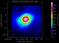
Make a 0th moment (integrated intensity) map using the task immoments and browse it using the viewer.
# In CASA
immoments(imagename=blimagename,
    moments=[0],
    axis='spectral',
    chans='8~61',
    outfile=integimagename)

viewer(integimagename)
Imaging the Amplitude Calibrator and Measure the Value of Jy/K
Determination of the Jy/K conversion factor is achieved by imaging a source whose continuum flux is known and measuring the observed brightness temperature. One observation of this source - the amplitude calibrator - was made per day, giving a total of four datasets (see top).
The true size of the beam (point spread function), on which the Jy/K value depends, in a map is determined be several ingredients.
- The intrinsic beam size is determined by the antenna diameter and optics (and of course wavelength). Here we assume the intrinsic beam size of 1.13*lambda/D, where D=12 [m] is the diameter of the antennas, and the factor 1.13 is derived from the optics design of the ALMA 12-m antennas.
- The effective beam size is broadened by the following causes:
- The scanning pattern used to observe the map (i.e., sample spacing in both directions).
- The method used to grid the individual spectra into a map/cube.
The Analysis Utilities provides several tools to get estimates of these.
It is not necessary, but If you wish to try this out for yourself, you will first need to download the raw amplitude calibrator data file M100_Band3_TP_ampcal_UncalibratedData.tgz. How to obtain the data is described at M100_Band3#Obtaining the Data. Once you have unpacked the data you will have a directory called M100_Band3_TP_ampcal_UncalibratedData. In this directory, execute the scripts for individual datasets (A002_X85c183_X895.ms.scriptForSDampcalReduction.casa5p1.py, A002_X8602fa_Xc3.ms.scriptForSDampcalReduction.casa5p1.py, A002_X864236_Xe1.ms.scriptForSDampcalReduction.casa5p1.py, and A002_X86fcfa_X3ae.ms.scriptForSDampcalReduction.casa5p1.py) to calibrate, image and derive Jy/K factors of all four calibrator datasets. The general approach is almost identical to that of calibrating the science target data, with the exception of the baselining step. Then, Jy/K values are derived from the peak of temperature in images and stored in text files (with the suffix, '.jyperk.txt').
# In CASA
import analysisUtils as aU
es = aU.stuffForScienceDataReduction()
execfile('A002_X85c183_X895.ms.scriptForSDampcalReduction.casa5p1.py')
The Calibration Jy/K values are determined as follows. Note that the values for individual antennas are averaged for each day, each SPW, because the antennas used for the Science observations were not necessarily available for the corresponding amplitude calibrator observations.
#Date        Amp_Cal_Dataset           SPW17   SPW19   SPW21   SPW23
2014-07-01   uid___A002_X85c183_X895   41.52   42.47   43.58   42.98
2014-07-05   uid___A002_X8602fa_Xc3    41.17   42.77   39.83   41.85
2014-07-07   uid___A002_X864236_Xe1    39.64   42.20   39.94   40.57
2014-07-17   uid___A002_X86fcfa_X3ae   43.65   43.83   42.21   43.22
Combination with 12m and 7m Array Data
If you wish to learn how to combine the Total Power data with interferometric 12m and 7m data, see the guide for Data Combination M100_Band3_Combine_4.3
