Simulation Guide for New Users (CASA 3.3)
↵ Simulating Observations in CASA
This guide is applicable to CASA version 3.3. For simulation instructions for older versions of CASA see Simdata New Users Guide (CASA 3.2).
To create a script of the Python code on this page see Extracting scripts from these tutorials.
Explanation of the guide
When planning an interferometric observation it is useful to simulate the output of the instrument under a variety of conditions. In CASA, interferometric observations can be simulated using task sim_observe and quickly analyzed using task sim_analyze. This guide will demonstrate how to simulate an ALMA observation using these tasks. (Task sim_observe can also be used to simulate observations with other interferometers, but this currently requires advanced techniques not covered here.)
We begin with an image similar to something that might be observed with ALMA. We show how to rescale the image and specify the ALMA antenna configuration. We produce a simulated set of visibility measurements and then produce an image from the visibility data. In the process, we also generate useful figures to help us analyze the simulated output.
We will assume throughout only a general knowledge of interferometry and no specific knowledge of CASA.
Getting Started
The two things you need to get started are
- The image we will work with, and
- CASA version 3.3.
We will use the Spitzer IRAC 8 micron image of 30 Doradus, which you can download from the Simulation Inputs CASA Guide page.
To install CASA, follow the instructions given on the Obtaining CASA page.
CASA Basics
CASA is the post-processing package for ALMA and EVLA and can handle both interferometric and single dish data. Because sim_observe and sim_analyze are tasks within CASA, we start here with a brief introduction to some CASA basics. To learn much more about CASA, go to the CASA homepage. Walk-throughs of CASA data reduction for a variety of data sets can be found on the CASA Guides website.
Once you have installed CASA, you can launch it by typing "casapy" at the prompt or by double-clicking on the icon, depending on your system and preferences.

To see a list of all available CASA tasks, at the CASA prompt type
tasklist
To look at the inputs for an available task, use "inp". For instance
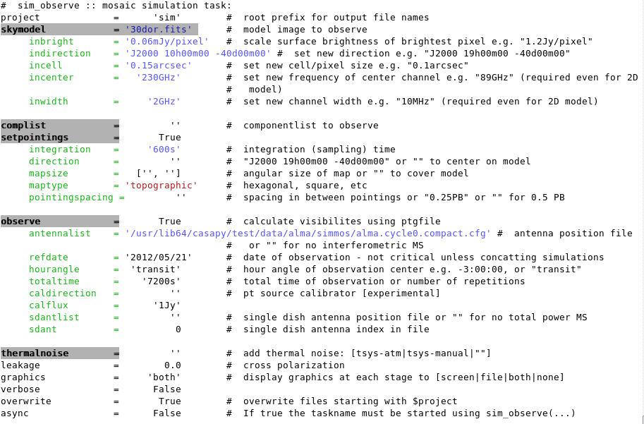
inp sim_observe
Any parameter with a grey background is expandable. Black text shows a default value. Red text shows an invalid value. Blue text shows a valid value different from the default.
To get help on a given task, use "help" (to exit from help, hit the "q" key). For instance
help sim_analyze
To reset a task to its default values, use "default". For instance
default sim_observe
To run a task using the current global values of its input parameters, just type its name at the CASA prompt. For instance
sim_observe
It's a good idea to double-check these values (i.e., re-run inp sim_observe) immediately before running a task.
Using sim_observe
The task sim_observe uses a model image along with a number of input parameters that define the observational conditions and alter the input model. The output of sim_observe is a visibility measurement set and various diagnostic plots and images.
Getting Your Input Image Into sim_observe
First, we'll tell sim_observe where to find the model (input) image and how to scale it appropriately for our purposes. Just to be safe, we'll begin by restoring the default values of sim_observe and then set the 30 Doradus image as the skymodel (Note: you might need to include the path to your model image, if you are not currently in the working directory where the image is).
#In CASA
default sim_observe
skymodel = '30dor.fits'
Angular Scale
If you open the FITS image of 30 Doradus in your favorite viewer (e.g. viewer in CASA), you will see that it covers quite a large footprint on the sky, about 10' on a side. We are going to tell sim_observe to rescale the pixels to shrink the image by roughly a factor of 15 (from 2.3" to 0.15" pixels through the incell parameter) so that the model is approximately 40" on a side. This rescaled model will fit within a small mosaic of 6 pointings. Although we do this primarily for convenience in this example, a scientific motivation for this type of rescaling would be to approximate what a super-giant HII region like 30 Doradus would look like if moved from the Large Magellanic Cloud to the distance of M33 or M31. For the sake of demonstration, we will also change the coordinates of the center of the map (using the indirection parameter). Units are case sensitive, so please take care to enter them in verbatim. CASA will throw an error otherwise.
#In CASA
incell = '0.15arcsec'
indirection = 'J2000 10h00m00 -40d00m00'
Observed Wavelength
The model image of 30 Doradus shows 8 micron continuum emission. ALMA does not observe at wavelengths this short, so we will tell sim_observe that this is actually a 230 GHz (1.3 mm) continuum map. We will also tell sim_observe that the observations were taken with a 2-GHz bandwidth. Although for this particular example the channel width is not a critical number, it would be very important if we were modifying a spectral cube instead of a continuum image.
#In CASA
incenter = '230GHz'
inwidth = '2GHz'
Brightness Scale
The 8 micron emission is probably not a great approximation for the millimeter emission from 30 Doradus. For a true science case, one would want to calculate what the expected 230 GHz emission would be from an object like this at the distance of about 750 kiloparsec. For the sake of simplicity, we will rescale the image so that the brightest pixel in the map has a flux density of 0.06 mJy. This number is chosen such that the extended emission is a factor of a few brighter than the expected noise in a 2 hour observation. The ALMA sensitivity calculator can be used to determine the expected noise for an observation.
#In CASA
inbright = '0.06mJy/pixel'
Remember that you can check your task inputs at any time by typing inp at the casa prompt.
Defining the Mock Observations
Now that sim_observe knows how to interpret the input image, the next step is to define the simulated observations.
Pointings and Scan Time
We will first change the parameters within setpointings.
The default value for integration, 10 seconds, might be appropriate to simulate real observations. However, sim_observe will run much faster if the value for "integration" is increased, reducing the number of data points to be generated. In this demonstration we will set it to 600 seconds. When sim_observe is used for scientific purposes it may be best to set integration to a large value at first to make sure that sim_observe runs as expected, and then decrease integration to a more realistic time for the final run. You will get a more accurate simulation with 10 second integrations than with 600 second integrations, especially in Early Science observations with a limited number of baselines.
#In CASA
integration = '600s'
Note that the integration time is different than the total (on-source) time of the observations. The integration time, set here, is the averaging time for each data point. The total time spent on-source is set below. Each pair of antennas will generate a number of data points equal to the total observing time divided by the integration time.
We will keep direction at the default (blank) value to center the observations on the model coordinates, as given in indirection above.
We will keep mapsize at the default value so that the mosaic will automatically cover the entire image. In our case, this will require a mosaic of 6 pointings (as we will see later on). One could also set an exact output image size via mapsize = ['10arcmin','10arcmin'] for example.
The default mosaic pattern, maptype = 'ALMA', tells sim_observe to use the same hexagonal algorithm as the ALMA OT. We will leave this unchanged.
Finally, we will also leave pointingspacing to its default value (blank), which automatically sets the pointings to be half a primary beam apart, corresponding to Nyquist sampling.
Antenna Positions and Total Observation Time
We will now consider the subparameters available when observe = True. We will keep the default values for every parameter (including totaltime = 7200s) except antennalist, which tells sim_observe the locations and sizes of each antenna in the array. We will simulate an Early Science observation, so we will first find the location where CASA has stored the ALMA configuration files. Then we will tell sim_observe to use the configuration file designed for Early Science.
#In CASA
repodir = os.getenv("CASAPATH").split(' ')[0]
antennalist =  repodir+"/data/alma/simmos/alma.cycle0.compact.cfg"
The first line, run within CASA, uses a Linux command to determine the path for CASA. The second line sets the antennalist parameter to the Early Science configuration. Other .cfg files in the same directory exist for various ALMA Full Science array configurations as well as the configuration files for other radio interferometers.
Most of the other parameters are not relevant for this simulation as we are not using a component list to describe the sky emission, we do not want to simulate observations of a calibrator, and we do not want to simulate single dish observations. Note that at this stage of simulation development, the time portion of the refdate parameter is ignored and all observations are instead centered around transit on the date specified.
Thermal Noise
For this simple simulation, we will not include any thermal noise in the observations, so we can leave thermalnoise at its default (blank) value.
sim_observe Execution and Output
With all the input parameters set, we are ready to execute the task:
#In CASA
sim_observe()
All sim_observe output will be written to a directory whose name was given by the project parameter, in our case, project = 'sim'. Inside this directory, you will find

- The simulated measurement set (sim.ms),
- a CASA image of the point spread function (sim.quick.psf),
- a CASA image of the input sky model rescaled according to the skymodel sub-parameters (sim.skymodel),
- a flattened CASA image of the input sky model rescaled (sim.skymodel.flat),
- a flattened PNG image of the input sky model rescaled and overlaid with the mosaic pattern specified by the setpointings sub-parameters (sim.skymodel.png),
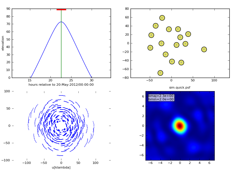
- a 2x2 PNG summary plot (sim.observe.png) showing,
- source elevation vs. time,
- antenna position,
- uv coverage,
- and the point spread function,
- and an ASCII text listing of mosaic pointings.
When sim_observe is executed, the 2x2 PNG plot will be displayed in the CASA plotter.
Using sim_analyze
Now that sim_observe has created a simulated set of visibility measurements, we are ready to image the visibilities and analyze the result. The task sim_analyze has been created to easily perform the imaging and subsequent generation of useful analysis plots and figures. We begin by resetting the sim_analyze inputs to their default values.
#In CASA
default sim_analyze
We next setup the imaging and analysis input parameters.
Image
We want to make a deconvolved output image, but we don't want to spend too much time optimizing the cleaning. So, all we need to do is make sure the "image" parameter is set to True (which it is by default) and leave all of its sub-parameters at their default values. Other data reduction guides describe the process of imaging in greater detail.
For simulations intended for a proposal or scientific analysis, one would almost certainly want to choose a more appropriate cleaning threshold and define the region to be cleaned. Instructions for how to define the region to be cleaned with the "mask" parameter can be found by typing
> help clean
or by looking at the Clean CASA Guide page.
Analyze
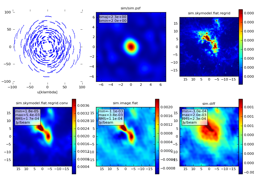
To specify how sim_analyze displays the imaged data, set the parameter "analyze" to True and then pick your favorite output formats. If the graphics parameter is set to 'screen' or 'both', up to six output formats will be displayed in the CASA plotter. More than six outputs can be written to disk (graphics = 'file' or 'both'), but only six can be displayed in the plotter. In this example we will look at,
- the uv coverage in the 2 hour observation,
- the synthesized beam (point spread function),
- the original sky model (as defined in "modifymodel"),
- the convolved model (sky model convolved with the synthesized beam),
- the clean image (the sky as observed with the interferometer after deconvolution),
- and the difference between the clean image and the convolved model.
To make these choices, use the following lines in CASA
#In CASA
analyze = True
showconvolved = True
showfidelity = False
sim_analyze Execution and Output

Execute sim_analyze by typing,
#In CASA
sim_analyze()
The six outputs we selected will be displayed in the CASA plotter and written to disk in the sim directory.

All CASA images written to disk can be opened later using the CASA viewer. Just type
> viewer
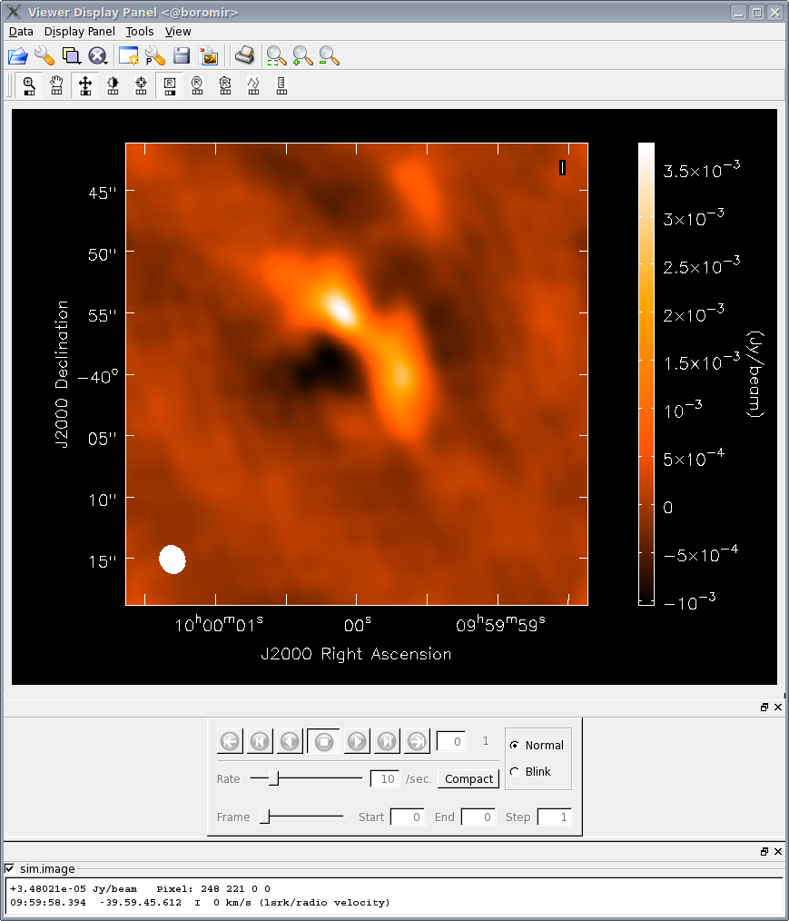
at the CASA prompt to start the viewer tool, and navigate to the appropriate directory, in our case sim. To display the simulated observations, first click on sim.alma.cycle0.compact.image, then click the "raster image" button and then click "done". The image will be shown in the viewer, and clicking on the picture of the wrench in the upper left corner will allow you to alter the image in many ways, such as changing the color scale, changing the coordinate scale, and axis labels. The image to the right was created by:
- changing basic settings -> color map from "Rainbow 2" to "Hot Metal 1",
- changing beam ellipse -> beam style from "outline" to "filled",
- and changing color wedge -> display color wedge from "No" to "Yes".
You can learn much more about the functionality of the CASA viewer by watching this instructional video.