Image Continuum CASA 6.1.1
This guide should be used after completing Prepare the data for Imaging. You should have created calibrated_final.ms prior to proceeding. Commands for this guide can be found in scriptForImaging_template.py available on github.
Check CASA version
This template is for use in CASA versions 4.4 and greater. The following code checks the version of CASA and exits if it is less than 4.4.0. You can download the appropriate version of CASA from Obtaining CASA . See Prepare for Imaging section on the main page of this guide for more information.
# in CASA
import re

if casadef.casa_version < '4.4.0' :
    sys.exit("Please use CASA version greater than or equal to 4.4.0 with this script")
Create an Averaged Continuum MS
<figure id="Calibrated_final_Field0_Spw0.png">
</figure> <figure id="Calibrated_final_Field0_Spw3.png">
</figure>
Appropriate averaging of a measurement set can reduce overall data volume, making imaging faster with clean. Since the continuum image is formed by essentially summing the entire bandwidth, we can spectrally average the input measurement set prior to imaging without significantly affecting the final imaging results. Below, we outline a procedure to create a spectrally averaged measurement set for continuum imaging.
The first step is to identify which spectral windows (spws) you would like to include in the continuum. In general, you should include all spws with bandwidths greater than 250MHz to maximize the available continuum bandwidth. Once you have determined which spws you would like to use to form the continuum ms, set the contspw variable:
# in CASA
# Set spws to be used to form continuum
contspws = '0,1,2,3'
The next step is to identify and flag the spectral lines in all spectral windows that you will use to make the continuum image. You will split and average the data with the spectral lines flagged so that your final spectrally averaged continuum ms only contains continuum emission. Two methods commonly used to identical spectral line emission are: 1) a channel vs. amplitude plot of the visibilities and 2) a dirty image of the cube.
To use the first method, create a channel vs. amplitude plot using plotms. An example command is given below. You may wish to change the averaging and the uvrange to identify extended emission.
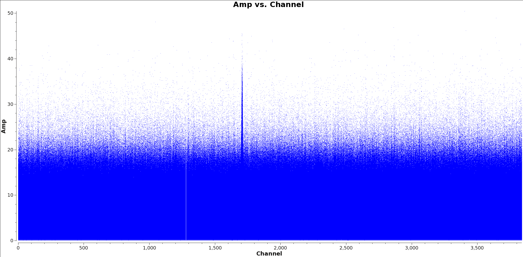
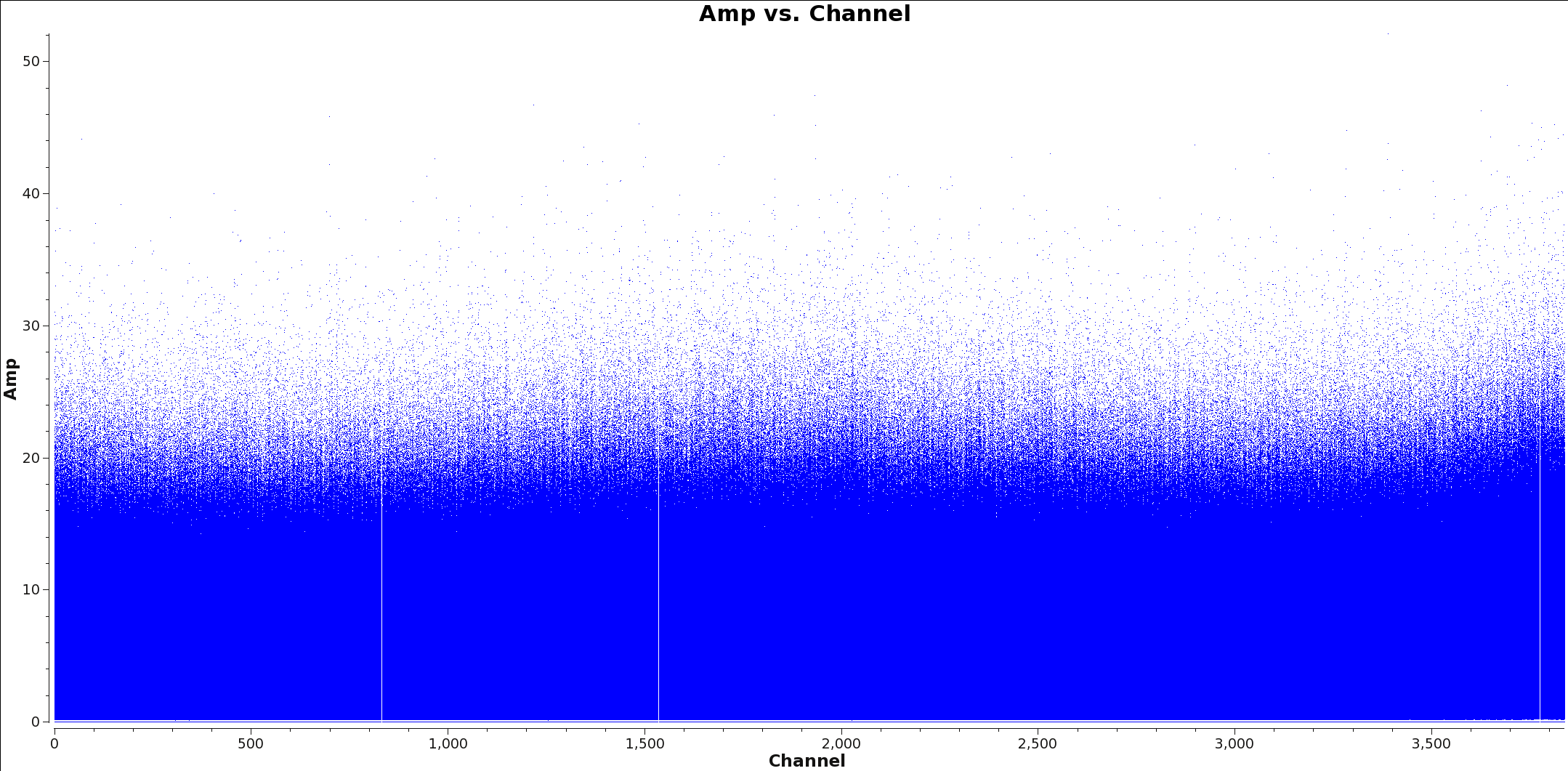
Figures 1 and 2 show example plots of an spw without a line to flag (Figure 2) and a line which you would need to flag (Figure 1).
Warning: If you apply channel averaging greater than 1, the numbers displayed on the channel axis will represent the channel bin number, rather than the averaged channel.
# in CASA
plotms(vis=finalvis, xaxis='channel', yaxis='amplitude',
   	ydatacolumn='data',
   	avgtime='1e8', avgscan=True, avgchannel='1',
   	iteraxis='spw' )
The second, and more accurate, method is to use clean to make a quick dirty image cube of channels with niter set to zero and mode=’channel’. Inspecting this channel cube for line emission gives a better defined channel range to flag. The basic command to create dirty image cubes is given below. This command should be repeated for each spw and science field.
#In CASA

testimagename=’testImage’
field=[‘0’] #list all target fields
spw=[‘0,1,2,3’] #list all target spw’s

for i in field:
      for j in spw:
            clean(vis=finalvis,
            	  imagename=testimagename+’Field_’+str(i)+’_spw_’+str(j),
            	  field=str(i),
      	          spw=str(j),
	          #      phasecenter=phasecenter, # uncomment if mosaic.
      	          mode='channel',
      	          outframe=outframe,
      	          niter=0,
      	          interactive=True,
      	          cell=cell,
      	          imsize=imsize,
      	          weighting=weighting,
      	          robust=robust,
      	          imagermode=imagermode)
<figure id="Wt_vs_Freq_spw0123.png">
</figure>
The first step to flagging the spectral line channels in your data is to use the flagmanager task to save the state of the data before any flagging is applied. You will need to revert back to the non spectral line flagged dataset when line imaging is done later on. In addition, if you accidentally flag any data you can easily correct this by restoring the before_cont_flags file using the flagmanager.
# in CASA
flagmanager(vis=finalvis,mode='save',
versionname='before_cont_flags')
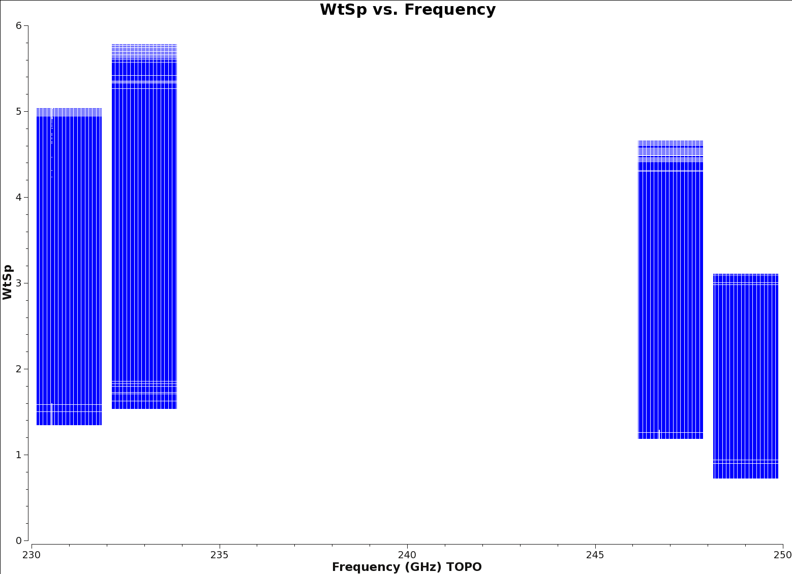
Initialize the per-channel (or spectral) weights in the ms using initweights. This step ensures that when the flagged and unflagged channels are combined, the appropriate weighting is given to the final set of averaged channels. Figure 3 shows a representation of the weightspectrum vs. frequency plot you should see after initializing the spectral weights
# in CASA
initweights(vis=finalvis,wtmode='weight',dowtsp=True)
The exact spectral window and channel ranges to flag in the flagchannels variable needs to be specified. For example, if spws 2&3 have a line between channels 1201 and 2199 and spectral windows 0 and 1 are line-free the command would be:
# in CASA
flagchannels='2:1201~2199,3:1201~2199' # modify the channel range for your dataset
<figure id="Calibrated_final_field0_spw0_LineChannelFlagged.png">
</figure>
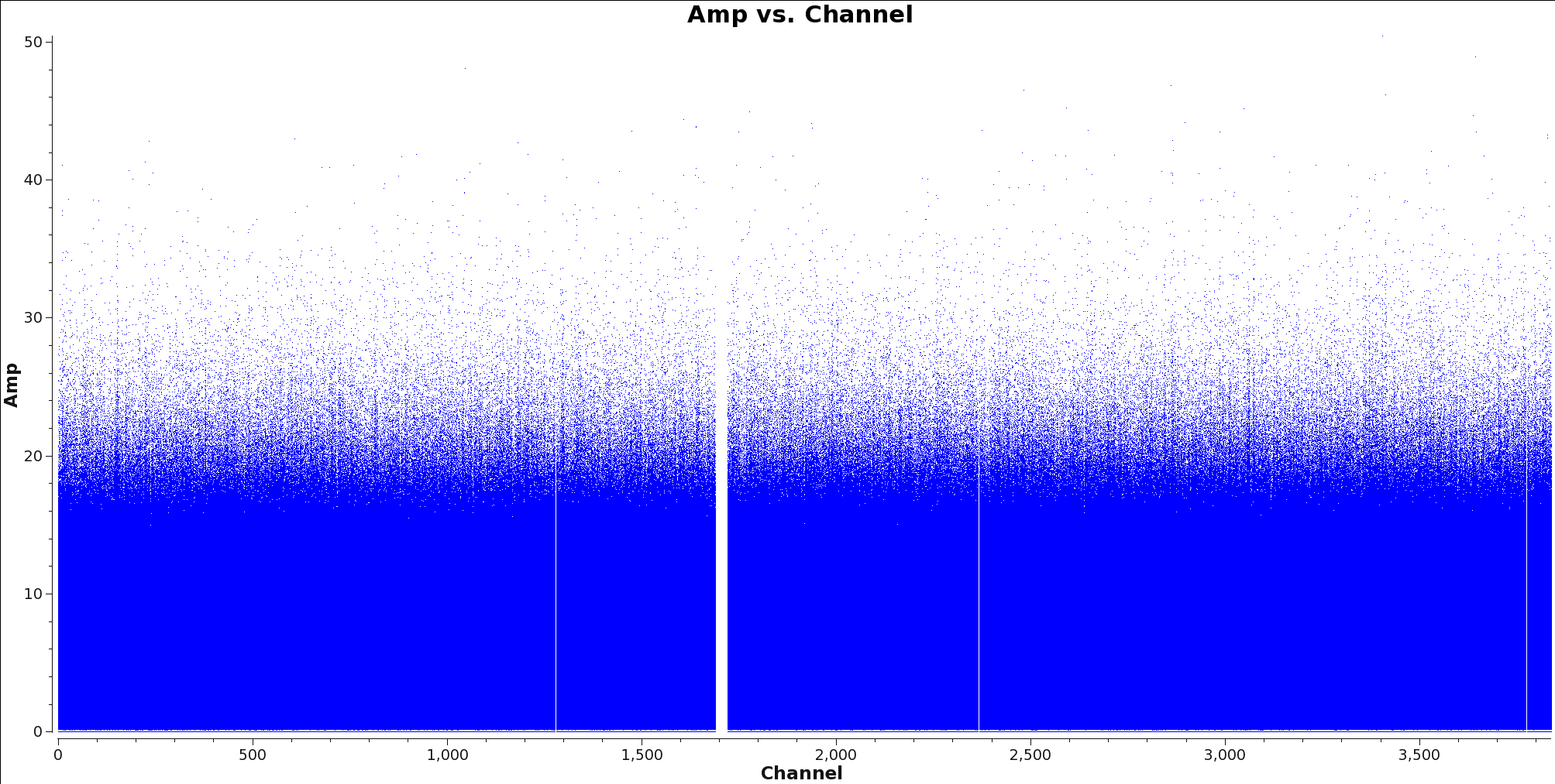
Next, use the task flagdata to apply these flags. After this is done, check that the flags were applied correctly by using plotms to inspect the flagged ms. Figure 4 shows an example of what you should expect to see.
# in CASA
flagdata(vis=finalvis,mode='manual',
      	spw=flagchannels,flagbackup=False)

# check that flags are as expected, NOTE must check reload on plotms
# gui if its still open.
plotms(vis=finalvis,yaxis='amp',xaxis='channel',
   	avgchannel='1',avgtime='1e8',avgscan=True,iteraxis='spw')
Now we can spectrally average the channels together to reduce the size of the continuum ms. The number of channels that we can average together is limited by what is referred to as "bandwidth smearing". When creating an interferometer image, we assume that the emission is essentially monochromatic. If we average large numbers of channels together, this is no longer an appropriate assumption and results in radial smearing in the image that increases in magnitude from the delay tracking center. For a detailed discussion, consult Bridle and Schwab, 1999, Synthesis Imaging in Radio Astronomy II, 180, 371. For a short derivation of the relevant quantities, see How to Calculate Bandwidth Smearing. Conservative values for averaging channels in various ALMA bands are suggested below. As a rough guide, the number of channels you can average together is:
- Bands 3, 4, 5, and 6: 125MHz/ (Channel Width (MHz))
- Band 7: 250MHz/ (Channel Width (MHz))
In general, you should make sure that the number of channels you are averaging together is an integer multiple of the original total number of channels. For example, if you have 128 channels and a channel width of 15.625 MHz in band 6, you can average together 8 channels at a time. The resulting ms will contain 16 final channels each with a channel width of 125MHz.
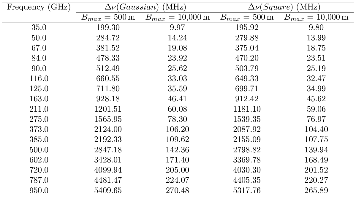
This table lists the maximum bandwidth allowed for a reduction in peak response to a point source over the field of view of 1% for a a square and Gaussian bandpass for various observing frequencies and baselines for different two bandpass types.
Finally, the task split is used to average the channels together to produce the spectrally averaged continuum data set.
# in CASA
contvis='calibrated_final_cont.ms'
rmtables(contvis)
os.system('rm -rf ' + contvis + '.flagversions')
split2(vis=finalvis,
 spw=contspws,
 outputvis=contvis,
 width=[8,8,8,8], # number of channels to average together. The final channel width should be less than 125MHz in Bands 3, 4, and 6 and 250MHz in Band 7.
 datacolumn='data')
Now you should check the weights of the new continuum measurement set. The ratio of the weights value between Time Domain Mode (TDM) and Frequency Domain Mode (FDM) windows should be approximately equal to the ratio of the channel widths. In addition, any heavily flagged channels should have their weights scaled by the ratio of the unflagged bandwidth to the bandwidth per output channel. For more information about data weights, see the Data Weights and Combination guide.
# in CASA
# update the antenna and field parameters for your dataset
plotms(vis=contvis, yaxis='wtsp',xaxis='freq',spw='',antenna='DA42',field='0')
Finally, we need to use the flagmanager tasks to restore the ms file to its original unflagged state, so that later we can do continuum subtraction and line imaging.
<figure id="Amp_vs_uvdist.png">
</figure>
# in CASA
# If you flagged any line channels, restore the previous flags
flagmanager(vis=finalvis,mode='restore',
        	versionname='before_cont_flags')
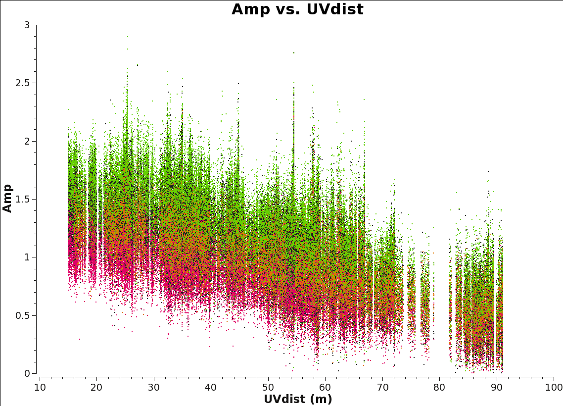
It is a good practice to inspect the final continuum ms to make sure that it is correct. In general, the distribution of amplitude vs. uv distance should be smooth. Recall this plot will be a horizontal line for a point source, while the short uv-distances will have higher amplitudes for a more extended object.
# in CASA
plotms(vis=contvis,xaxis='uvdist',yaxis='amp',coloraxis='spw')
Image Parameters
Before imaging, you should set a few key parameters that you will use throughout the rest of the script.
Set the field id for the science target you are interested in imaging. You can use the listobs file generated during the imaging prep step to find this information. If you are imaging a mosaic then you will have to select all the fields. For example, field = ‘3~25’. You can also set the field variable to the name of the source, as long as it matches the name in the listobs file. Do not leave the field parameter blank. If you leave the field parameter blank, clean will attempt to image all sources in the measurement set.
# in CASA
# update for your ms
field='0'
Uncomment the imagermode that is relevant to your dataset. Set the phase center by field id or coordinates if you are imaging a mosaic. Check the spatial setup in the weblog (for pipeline calibrations) or qa2 report (for manual calibrations) to find the phase center. You should choose the central field for the phase center in order to get the best results.
If you are unsure which field to use for the phase center after looking at the weblog then you may use the following Analysis Utilities command:
au.pickCellSize(‘calibrated_final.ms',imsize=True).
This will return a four element array with that contains the calculated cell size, the X axis number of pixels, the Y axis number of pixels, and the field number that is most centered in the mosaic. You may use this as the phase center field id in your script. If you haven't installed Analysis Utilities, see the | Obtaining Analysis Utilities section for instructions.
Another method of finding the central field number uses the plotmosaic Analysis Utilities au.plotmosaic(‘calibrated_final.ms’). This method will produce a plot of all fields with their corresponding field numbers plotted on the sky. You can also set the phase center with the coordinates at the center of this plot.
# in CASA
# imagermode='csclean' # uncomment if single field
# imagermode='mosaic' # uncomment if mosaic or if combining one 7m and one 12m pointing.
# phasecenter=3 # uncomment and set to field number for phase
            	# center. Note lack of ''.  Use the weblog to
            	# determine which pointing to use. Remember that the
            	# field ids for each pointing will be re-numbered
            	# after your initial split. You can also specify the
            	# phase center using coordinates, e.g.,
            	# phasecenter='J2000 19h30m00 -40d00m00'
<figure id="Calibrated_final_AmpVsUVWave.png">
</figure>
Next you will determine the cell (or pixel) size. To do this, you need to determine the approximate resolution of your observations. Then you divide the resolution in arcsec by 5 to 8 to adequately sample the PSF. The resolution of a particular interferometer observations can be estimated from the length of the longest baseline:
resolution (radian) ~ (observed wavelength) / (length of longest baseline)
If the baseline is measured in wavelengths, this becomes
resolution (radian) ~ 1.0 / (length of longest baseline in wavelengths)
To convert from radians to arcsec, we multiple by 206265.0 to obtain:
resolution(arcsec) ~ 206265.0/(longest baseline in wavelengths)
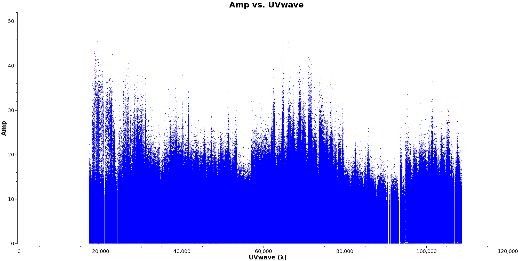
To determine the longest baseline in wavelengths use plotms with xaxis=’uvwave’ and yaxis=’amp’ on your ms file. Figure 1 shows an example of this plot. It is generally better to oversample your beam than to undersample, particularly for observations with poor uv-coverage.
cellsize(arc seconds) = resolution(arcsec)/5
The next step is to determine the image size in pixels. There are two methods of doing this depending on if you are imaging one field or a mosaic.
If this is a single field, the image size can usually be approximated to be the same size as the primary beam of the telescope. The ALMA 12m primary beam in arcsec scales as 6300 / nu[GHz] and the ALMA 7m primary beam in arcsec scales as 10608 / nu[GHz], where nu[GHz] is the sky frequency. However, if there is significant point source and/or extended emission beyond the edges of your initial images, you should increase the imsize to incorporate more emission.
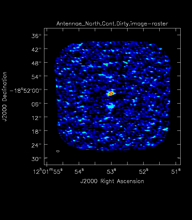
For mosaics, make the image substantially larger than the mosaic footprint. Use au.plotmosaic(finalvis) to find the mosaic footprint in arcseconds. Padding the imsize substantially avoids artifacts in the image. To know if you have padded enough you should, in your images, be able to see the edges of the outside fields being cut off. <figure id="Antennae_Antennae_North.Cont.Dirty.image.png">
</figure> <figure id="Antennae_North.Cont.Dirty.smallIMSize.image.png">
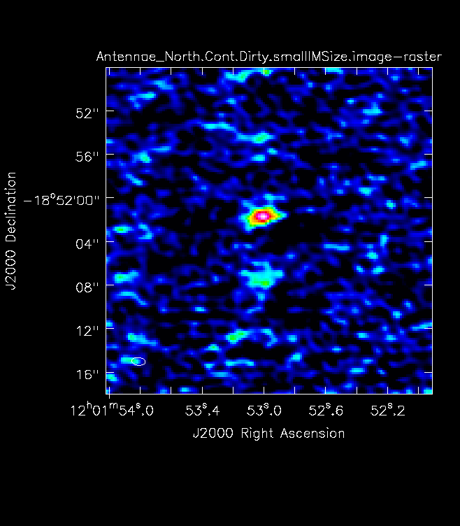
</figure> Note that the imsize parameter is in PIXELS, not arcsec, so you will need to divide the image size in arcsec by the pixel size to determine a value for imsize.
If you would like to check any of these calculations you may use the following command, au.pickCellSize('calibrated_final.ms', imsize=True), in CASA. This will return a four element array of the calculated cell size, the x axis imsize, the y axis imsize, and the central field id number.
# in CASA
cell='1arcsec' # cell size for imaging.
imsize = [128,128] # size of image in pixels.
When imaging you will need to set two specific velocity parameters called outframe and veltype. Outframe is the coordinate system used for the observation. If you have access to the original proposal, this can be found in the Observing Tool (OT) under field setup. A list of acceptable outframes that can be used in CASA can be found at https://help.almascience.org/index.php?/Knowledgebase/Article/View/86/0/what-are-the-frequency-reference-frames-in-casa. Note: heliocentric(hel) is deprecated in CASA. Use barycentric(bary) in this case.
You will also have to set the veltype for the clean command. This variable has only two options available, radio and optical. It is standard to leave this set to ‘radio’ in all projects regardless of the velocity frame used in the project.
# in CASA
outframe='bary' # velocity reference frame. See science goals.
veltype='radio' # velocity type.
The last four parameters that must be set are associated with how clean will weight and clean the data. During the imaging process, the individual visibilities are placed on a uv grid and then combined. Weighting determines how clean will combine the uv gridded to produce an image. There are several weighting schemes that can be used:
- Natural: Each cell in the uv plane is weighted by the number of points in the cell. This weighting scheme is the default in clean. It results in a lower noise image at the expense of worse angular resolution.
- Uniform: Each cell in the uv plane has the same weight. In this case, the sidelobes will be reduced because the imaging plane is filled in more uniformly. This weighting scheme also gives more weight to longer baselines resulting in higher resolution at the expense of higher noise. It can emphasize visibilities with calibration errors.
- Briggs: This weighting scheme is a combination of natural and uniform weighting. The weighting is controlled by the robust parameter. A robust parameter of 2 gives natural weighting, -2 uniform weighting, and a number in between a combination of natural and natural. Refer to Brigg's Thesis for more information. Currently, robust is set to 0.5 which gives a good compromise between natural and uniform weighting. You may find, after imaging, that you have to decrease the noise or angular resolution based on the desired performance requested in the proposal. Playing with the robust parameter can affect your final noise in the image and also the angular resolution.
The parameters niter and threshold provide two ways to stop the clean process. The niter parameter is the maximum number of iterations allowed. After this limit has been reached, clean will terminate. The threshold parameter sets a flux density threshold for the clean. When the peak residual is below this value, clean terminates. When cleaning interactively, we recommend setting the niter parameter to a large, but not too large value (say 10000 or 100000) so that clean terminates eventually in the case of human error. The threshold can be left at the default of 0.0mJy for interactive clean. For non-interactive clean, the recommendation is to set the threshold to several times the noise in the final image. To determine the threshold for cube images, run clean with niter set to zero and inspect the resulting image in the viewer. In a line-free channel, select a region and look at the statistics panel to determine the noise level. For more detailed instructions, see the “Image the Spectral Line Data” section of EVLA Spectral Line Imaging Analysis IRC+10216.
# in CASA
weighting = 'briggs'
robust=0.5
niter=1000
threshold = '0.0mJy'
For more information on the various options available in clean, refer to David Wilner’s Imaging and Deconvolution presentation from the 2016 Synthesis Imaging Workshop. The table below provides helpful pointers to relevant slides.
| Pixel and Image Size | Slides 40-41 |
| Weighting | Slides 42-48, 60-61 |
| Deconvolution Algorithms | Slides 50-53, 62 |
Imaging the Continuum
<figure id="Cont_before_clean.png">
</figure> <figure id="Cont_before_clean_mask.png">
</figure> <figure id="Final_Cont_residual.png">
</figure>
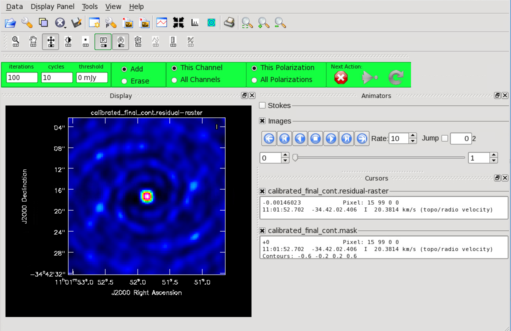
Now that you have set all of the imaging parameters, you will need in clean you can proceed to imaging the continuum. The First Look at Imaging CASAGuide gives an introduction to cleaning and imaging. We provide an abbreviated set of commands here. If you are imaging a mosaic, the phasecenter parameter should be set. Refer to the [#Image Parameters] section of this guide for instructions on how to determine this for your project. Type “help clean()” in CASA if you would like to explore the possible parameters of clean. Mode=’mfs’ sets the spectral gridding type to multi-frequency synthesis and creates a continuum image. Leave the psfmode to use during minor cycles at the default ‘clark’ . clean interactively as the threshold is set at 0 mJy. The mask parameter may also be added if you have an existing file.
# in CASA
contvis = 'calibrated_final_cont.ms'
contimagename = 'calibrated_final_cont'
# in CASA
clean(vis=contvis,
      imagename=contimagename,
      field=field,
#      phasecenter=phasecenter, # uncomment if mosaic.
      mode='mfs',
      psfmode='clark',
      imsize = imsize,
      cell= cell,
      weighting = weighting,
      robust = robust,
      niter = niter,
      threshold = threshold,
      interactive = True,
      imagermode = imagermode)
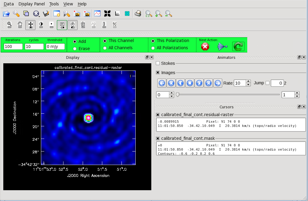
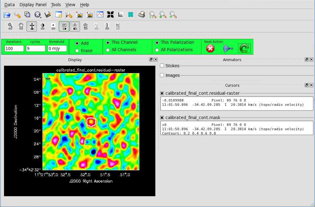
Figure 11 shows the clean GUI that will appear. If no source is apparent, no cleaning should be done. Press the red “X” to complete the task. If a source is apparent, create a mask around it using the mouse. Once a mask is created, the green arrow will be illuminated and you can begin the first round of cleaning. The logger window gives you vital information on the progression of clean. Once the cycle is complete, the residuals will appear in the GUI. You should continue to iterate until the region inside the mask matches the noise outside the mask. You may need multiple cycles depending on the complexity of the source.
The red "X" will stop clean where you are, the blue arrow will stop the interactive part of clean, but continue to clean non-interactively until reaching the number of iterations requested (niter) or the flux density threshold (whichever comes first), and the green circle arrow will clean until it reaches the "iterations" parameter on the left side of the green area. These are the only safe exit buttons to use during clean. DO NOT CTRL-C OR KILL CLEAN WHILE IT IS RUNNING. If you do this, it is very likely that your ms may be corrupted.
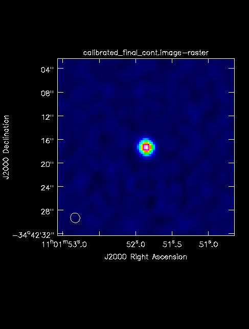
The final continuum image.
After creating the continuum image, check the noise and resolution to make sure the results match the expected values.
For each image it creates, clean generates several images with the name imagename+extension. If you re-run clean with the same imagename, clean will use the existing files as a starting point, continuing the clean where you left off. To start completely from scratch, either change the imagename or delete all the files from the previous clean run. Note that CASA retains some image information in memory, so to truly delete the images from open version of CASA, you need to run the rmtables command. See below for an example.
# in CASA
for ext in ['.flux','.image','.mask','.model','.pbcor','.psf','.residual','.flux.pbcoverage','.pb','.wtsum']:
	rmtables(contimagename+ext)
Once you are happy with your continuum image(s), you can continue to Self-Calibration Template or Spectral Line Imaging Template. If you do not wish to self-calibrate or create line cubes, continue with this guide to create primary beam corrected images and fits files.
Apply a primary beam correction
<figure id="TW_Hya_Calibrated_final.pbcor.png">
</figure>
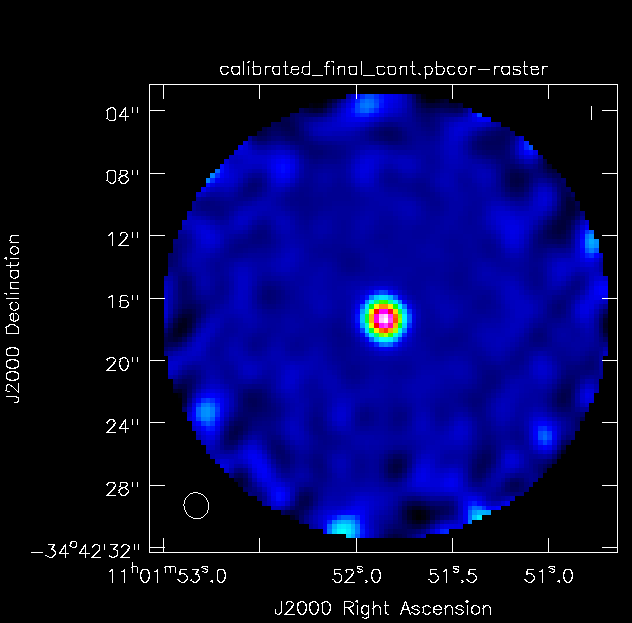
After the data have been cleaned, we apply a primary beam correction to the data. This procedure corrects the image produced by clean for the response function of a single antenna (i.e., the primary beam), or in the case of mosaics the sum of the response functions of all the pointings in the mosaic. The task impbcor is used to produce the primary beam corrected images . You will need the *.flux and *.image files produced by clean.
# in CASA
import glob

myimages = glob.glob("*.image")

rmtables('*.pbcor')
for image in myimages:
	pbimage = image.rsplit('.',1)[0]+'.flux'
	outfile = image.rsplit('.',1)[0]+'.pbcor'
	impbcor(imagename=image, pbimage=pbimage, outfile = outfile)
Export the images
Use exportfits to create fits files of the *.flux and *.pbcor files.
# in CASA
import glob

myimages = glob.glob("*.pbcor")
for image in myimages:
    exportfits(imagename=image, fitsimage=image+'.fits',overwrite=True)

myimages = glob.glob("*.flux")
for image in myimages:
    exportfits(imagename=image, fitsimage=image+'.fits',overwrite=True)
Create Diagnostic PNGs
The First Look at Image Analysis guide gives an introduction to a variety of options to begin image analysis, including using immoments to create moment maps. The following commands create png files of the continuum image.
<source lang="python">
- in CASA
os.system("rm -rf *.png") mycontimages = glob.glob("calibrated*.image") for cimage in mycontimages:
   max=imstat(cimage)['max'][0]
   min=-0.1*max
   outimage = cimage+'.png'
   os.system('rm -rf '+outimage)
   imview(raster={'file':cimage,'range':[min,max]},out=outimage)