DataWeightsAndCombination
Most recently updated for CASA Version 6.6.1 using Python 3.8
Introduction
The purpose of this guide is to describe the CASA visibility weights, and how they relate to data combination. If you are trying to combine ALMA data from Cycles 0, 1, and/or 2, you should be aware of the issues described here. Only data calibrated in >=CASA 4.2.2 pipeline, or manual reduction in >=CASA 4.3 are free from any issues. All of the data to be combined must be in a consistent weight state.
Principles of Data Weighting
Visibility Weights
For optimal imaging performance it is critical that in a relative sense each visibility in the data have the correct weight after calibration -- that is, data with better sensitivity have more weight than data with less sensitivity. Formally, the post-calibration visibility weights should be equal to 1/σij2 where σij is the rms noise of a given visibility.
[math]\displaystyle{ \sigma_{ij} (Jy) =\frac{2k}{\eta_{q}\eta_{c}A_{eff}} }[/math] [math]\displaystyle{ \sqrt{\frac{T_{sys,i} T_{sys,j}}{2\Delta\nu_{ch} t_{ij}}} }[/math] [math]\displaystyle{ \times 10^{26}, }[/math]
where:
k is Boltzmann's constant.
Aeff is the effective antenna area which is equal to the aperture efficiency (ηa) x the geometric area of the antenna (π r2). The aperture efficiency depends on the rms antenna surface accuracy and is about 0.75 for ALMA dishes.
ηq and ηc are the quantization and correlator efficiencies, respectively. These have values of about 0.88 and 0.96, respectively. See the ALMA Technical Handbook for more information.
Tsys,i is the system temperature for antenna i, and Tsys,j is the system temperature for antenna j
Δνch is the effective channel frequency width.
tij is the integration time per visibility.
Note, this equation can be extended from a single visibility to the expected imaging rms noise for one channel in an entire dataset by replacing Tsys,iTsys,j by the average Tsys2, tij by the total time on source, and the [math]\displaystyle{ \sqrt{2} }[/math] in the denominator by [math]\displaystyle{ \sqrt{N(N-1)} }[/math] , where N is the number of antennas. Additionally, [math]\displaystyle{ \sqrt{n_p} }[/math] is included in the denominator, where np is the number of polarizations (1 for single pol and 2 for dual or full pol data):
[math]\displaystyle{ \sigma_{image} (Jy) =\frac{2k}{\eta_{q}\eta_{c}A_{eff}} }[/math] [math]\displaystyle{ \sqrt{\frac{T_{sys}^{2}}{N(N-1)\Delta\nu_{ch} t_{source}n_{p}}} }[/math] [math]\displaystyle{ \times 10^{26}, }[/math]
In order to correctly combine and image data that have different Tsys, Δνch, tij, or antenna size it is essential to use visibility weights proportional to 1/σij2. The remainder of this guide deals with ensuring that the individual visibility weights are correct in your ALMA data.
Relative Overall Weights between Configurations
Additionally, when combining data from different antenna configurations, one will get optimal overall sensitivity to all spatial scales by matching the surface brightness sensitivity at each uv-distance. This can only be achieved by having time-on-source per configuration in the right proportion. This topic is covered in ALMA Memo 598. This memo informs the relative amount of time that ALMA observes a project with the 7m-array versus the 12m-array, and compact versus extended 12m-array configurations. However, since telescope time is expensive, one typically does not actually observe in the optimal proportion, in that case one will not fully realize the expected "impact" of adding the less sensitive configuration data. In that case, one may chose to "up-weight" the less sensitive configuration explicitly by changing its data weights, above and beyond 1/σij2. However, it should be noted that nothing comes for free, and such a change will come at the expense of overall image sensitivity though it may very well be the optimal choice for your science case -- for example, if you are particularly interested in large scale structures you might apply extra up-weighting to the dataset(s) with the shortest baselines. Finding the optimal up-weighting is a matter of experimentation, but can easily be explored using the visweightscale parameter in concat. As a general rule of thumb extra up-weighting by more than a factor of 4 or so is not recommended. Before experimenting with this however, its always best to start with data that simply has the correct 1/σij2 weights. Additionally, some degree of relative re-weighting can also be accomplished simply by using the Briggs Robust parameter, without explicitly changing the visibility weights, and generally it is also a good idea to try this first before more aggressive up-weighting is attempted.
Weights in CASA
Data weights are described in the CASA Docs here: dataweights
To summarize the situation specifically for ALMA data processed by the ALMA Project:
- Case 1) CASA 4.2.1 and earlier: Weights were calculated on a per spw bases and scaled by Nchan/[(Tsys(i) * Tsys(j)] using calwt=True at the applycal stage for Tsys table. Assuming that (i) there aren't any unflagged antennas with significantly low gain due to for example pointing errors, or hardware problems, and (ii) all the antennas have similar efficiencies -- usually good assumptions for ALMA data, then to good approximation the data weights are close to internally consistent and can produce good imaging results, but should not be combined with other data that have different Δνch, tij, or antenna size without further modification.
- Case 2) CASA 4.2.2 and later: Upon import data weights are scaled by 2ΔνchΔtij and then also scaled by 1/[(Tsys(i) * Tsys(j)] using calwt=True at the applycal stage for Tsys table (thus making them per channel weights). Additionally:
- (A) For data calibrated by the 4.2.2 CASA Pipeline the weights are further modified by [gain(i)2 * gain(j)2] when the amplitude gain table is applied using calwt=True. Since the amplitude gains are directly proportional to the effective Antenna area, scaling the weights by the amplitude gains will take into account antenna size differences, and also down-weight antennas with comparatively low gain. Thus, these weights are correct (but see #Absolute_Accuracy_of_the_Data_Weights).
- (B) For data manually calibrated in CASA 4.2.2, unfortunately calwt=False was still used to apply the antenna gain table, thus, these data have weights that are not correct in a relative sense when compared to other data with different antenna size by the factor [gain(i)2 * gain(j)2].
- Case 3) CASA 4.3 and later: Data calibrated in either the pipeline or manually will have correct weights (but see #Absolute_Accuracy_of_the_Data_Weights). An example of this situation is demonstrated in M100_Band3_Combine.
How Do I Know the Situation For My ALMA Data?
First, remember that good imaging performance requires that the relative weights be correct for all data included in the imaging. For all of the situations below, the data are sufficiently internally consistent that they can be imaged fine on their own or with other data that share the same situation and have the same data properties. Problems arise when data are combined that (a) do not share the same weight situation and/or (b) have differences in antenna size, visibility integration time, or channel bandwidth that are not accounted for.
All datasets to be combined should be independently assessed to determine their weight situation and thus whether corrective action is required
- Cycle 0 and Cycle 1 data were reduced in 4.2.1 or earlier versions and correspond to Case 1 above. ACA 7m-array data were first offered in Cycle 1. If you want to combine 12m-array and 7m-array data taken during Cycle 1, it is very likely you need to correct the visibility weights before imaging.
- Cycle 2 data has a more confused range of possibilities (this includes actual Cycle 2 projects and carry-over projects or parts of projects from Cycle 1). Recall from Case 2 above, that the key factor that determines your situation for Cycle 2 is whether the data were pipeline or manually calibrated.
- Key dates:
- Start Cycle 2: June 1, 2014
- CASA 4.2.2 release date: Sept. 4, 2014
- Pipeline release date: Oct. 20, 2014
- The earlier in Cycle 2 your data was taken, the more likely it was manually calibrated, also if you have any very narrow spws, high frequency, etc it is more likely data were manually calibrated.
- If the data were manually calibrated early in Cycle 2 it is likely in Case 1 (certainly the case for data earlier than Sept. 2014). After Oct. 1, 2014 it is likely to be in Case 2B.
- How can I distinguish between pipeline and manual data reduction for Cycle 2 data?
- In your data delivery, the README file should say but there were some oversights on this front. A sure way to tell: look in the directory called script within your data delivery for a particular member_ouss. If you see a file with PPR*.xml, the data was calibrated by the pipeline. Otherwise it was done manually.
- Key dates:
Checking the weights in your data
This section follows the M100_Band3_Combine guide. The data for this CASA guide has already had the weights corrected. We will illistrate how to check the weights in your data. You will need the data from this tutorial to complete this example.
To verify that the weights come out as expected, we plot the weights of the 7m and 12m data and measure their ratio to be, on average, 7m/12m ~ 0.055/0.3 ~ 0.18. Note that in the plots the points are colored by SPW, so there is only one 12m CO SPW but there are two 7m CO SPWs, and that no averaging can be turned on when plotting the weights.
# In CASA
os.system('rm -rf 7m_WT.png 12m_WT.png')
plotms(vis='M100_12m_CO.ms',yaxis='wt',xaxis='uvdist',spw='0:200',
       coloraxis='spw',plotfile='12m_WT.png',showgui=True)
#
plotms(vis='M100_7m_CO.ms',yaxis='wt',xaxis='uvdist',spw='0~1:200',
       coloraxis='spw',plotfile='7m_WT.png',showgui=True)
The two key things that are different between the 7m and 12m-array data are that the effective dish areas are different by (7/12)2, and the integration times are different by (10.1/6.05). Since the dish area and the integration time per visibility are in the denominator of the radiometer equation, and assuming the weight of an individual visibility is proportional to 1/sigma2, the ratio of the weights should be (7./12.)4 x (10.1/6.05) = 0.19. This is very close to the value we measure for the ratio of the weights, particularly given that the 7m flux calibration relied on a source which changed substantially over the course of the six 7m-array observations.
Now concatenate the two data sets and plot the concatenated weights to verify that they are as expected.

# In CASA
# Concat and scale weights
os.system('rm -rf M100_combine_CO.ms')
concat(vis=['M100_12m_CO.ms','M100_7m_CO.ms'],
       concatvis='M100_combine_CO.ms')

# In CASA
os.system('rm -rf combine_CO_WT.png')
plotms(vis='M100_combine_CO.ms',yaxis='wt',xaxis='uvdist',spw='0~2:200',
       coloraxis='spw',plotfile='combine_CO_WT.png',showgui=True)
Here, we create more instructive plots of the combined data to check that things are in order. (Let each plot finish before cutting and pasting next plot. If plotms gui disappears, exit CASA and restart.)
One way to assess the relative noise in the combined data is to plot amplitude as a function of uv-distance. Here, it's clear that the 7m data is noisier than the 12m data (note also that this plot is not shown):
# In CASA
os.system('rm -rf M100_combine_uvdist.png')
plotms(vis='M100_combine_CO.ms',yaxis='amp',xaxis='uvdist',spw='', avgscan=True,
       avgchannel='5000', coloraxis='spw',plotfile='M100_combine_uvdist.png',showgui=True)
A fairer comparison of these data is achieved by isolating the brightest line channels in individual 12m and 7m data sets (i.e., not the concatenated data sets) and comparing only those channels in amplitude vs. uv-distance. Here the agreement is better, as it is less dominated by the scatter among the several 7m executions.

To plot the CO line as a function of velocity (this plot takes a while):
# In CASA
os.system('rm -rf M100_combine_vel.png')
plotms(vis='M100_combine_CO.ms',yaxis='amp',xaxis='velocity',spw='', avgtime='1e8',avgscan=True,coloraxis='spw',avgchannel='5',
       transform=True,freqframe='LSRK',restfreq='115.271201800GHz', plotfile='M100_combine_vel.png',showgui=True)
To see each spectral window independently in plotms, run the command again but remove the call to "plotfile" and add " iteraxis='spw' ".
What Are the Options for Adjusting the Weights for Older Reductions?
If the data weights are not correct in ALL the datasets you want to combine there are three options to correct the situation. These different methods carry different levels of complexity depending on your situation. The situation can also be extra confusing if your data fall into multiple categories above. For example, it is not uncommon that in Cycle 2 the 12m-array data could be pipeline calibrated, but the 7m-array data done manually. Pay close attention to recommendations in Red and the Caveats for each option. If you suspect your data have been reprocessed or are unsure of the weights, use the example above to check the weights of all your data.
Option 1: Re-calibrate your data in CASA 4.2.2 or later
- ⇒ Option 1 is easiest to implement for Case 2B (Data observed in Cycle 2 manually calibrated in 4.2.2 or 4.3.1 with calwt=False for amplitude/flux gain table).
- All data imported in 4.2.2 (or later) will automatically adjust the weights by 2ΔνchΔtij. The Tsys application should also already be correct in your scripts. To correct for antenna size and weight by the gains you must change calwt=True for the amplitude table in applycal.
- Where do I make the calwt change?
- As described in your README file, you can obtain a fully calibrated measurement set by executing the scriptForPI.py. For manually calibrated data, within the script directory you will also find scripts with the format uid*scriptForCalibration.py, one for each execution for that Scheduling Block -- the sciptForPI.py actually executes these scripts, thus this is where any change must be made.
- Toward the bottom of the uid*scriptForCalibration.py scripts (typically Step 17 or 18) you will find a step called # Application of the bandpass and gain cal tables. Change the calwt=False in all of the applycal calls to calwt=True.
- Caveat 1: You must have the raw ALMA ASDM to run the scriptForPI.py (see the README file for more information).
- Caveat 2: Most (all except early Cycle 0) ALMA manual calibration scripts have within them the CASA version used to create the script. For example, if your manual calibration script includes the following, using any other version than 4.2.2 will give an error (even though using, for example, 4.3.1 would be fine in this case):
# In calibration script
if re.search('^4.2.2', casadef.casa_version) == None:
sys.exit('ERROR: PLEASE USE THE SAME VERSION OF CASA THAT YOU USED FOR GENERATING THE SCRIPT: 4.2.2')
- You must change the version number in the script to match the version you want to use or the script will not run.
- Caveat 3: Scripts from earlier than 4.2.1 are likely to have commands that make them incompatible to run directly in later versions of CASA. It may be difficult for a non-expert to update the uid*scriptForCalibration.py script(s) to current syntax.
Option 2: Make an approximate overall relative correction to your calibrated science target data:
- ⇒ Option 2 is easy to implement for Cases 1 and 2B, but is not as accurate as Options 1 or 3. However, it is typically adequate for most purposes, and is MUCH better than doing nothing.
- All ALMA data reduced in CASA should already have 1/Tsys2 weighting which accounts for many of the factors that make data from some baselines more sensitive than others within an individual dataset. If we assume that antennas with abnormally low gains (typically due to poor pointing, hardware failures) have already been flagged and all antennas meet the surface accuracy specifications, then the amplitude gains will be fairly constant from antenna to antenna, with the value dominated by the antenna size. Other parameters that can often be different between datasets include the Δνch, and tij.
- Thus, a reasonably good approximation for the relative weight scaling for data_a compared to data_b is:
- Case 1: (antenna_size_b/antenna_size_a)4 x (Δνch_b/Δνch_a) x (tij_b/tij_a)
- Case 2B: (antenna_size_b/antenna_size_a)4
- such an overall scale factor can be applied during the concat step using the visweightscale parameter. Note that because its a ratio, it doesn't matter if you use the antenna radius or diameter as long as you are consistent. An example is given below.
- Caveat 1: This option requires that the datasets to be combined have only one (unflagged) antenna size per dataset. If this is not the case, then Options 1 or 3 must be used.
- Caveat 2: This option also requires that both datasets to be combined are in the same weight situation (i.e. mixed Cases cannot be handled using simple overall relative scaling).
Option 3: Run the task statwt on your calibrated science target data
- ⇒ Option 3 is pretty easy to implement for both Cases 1 and 2B, and will account for (likely small) Gain variations from antenna to antenna within the individual datasets, whereas Option 2 does not. However, see Caveat 1, for very complex line emission it may be difficult to get a good result.
- This task attempts to assess the sensitivity per visibility and adjust the weights accordingly. It is very commonly used for VLA data (including the VLA pipeline).
- Caveat 1: One must limit the calculation to line-free channels using the fitspw parameter. For complex line projects this can be painful, however, typically the line-free channels are already known from the continuum subtraction, and can be reused here. However, it is best to run statwt before continuum subtraction, and it should always be run on the fully channelized data before any spectral averaging is applied.
- Caveat 2: statwt does not currently account for channel-dependent flagging. It is critical to explicitly avoid the edge channels for any TDM spws in the data (128 channels per spw) data using fitspw, (example: for a dataset with only TDM spws, fitspw='*,7~120' ).
Example of Correcting Weights Using Option 2 (Relative Scaling)


Below we show what could have been done to approximately correct the weights in the M100 Science Verification data (7m-array and 12m-array) if it was reduced in CASA 4.2.1 (or earlier), i.e. Case 1. If you would like to try this for yourself, you can download the 12m data processed in CASA 3.3 from the data download link at M100_Band3#Obtaining_the_Data.
In CASA 4.2.1 and earlier, the data weights are 1 upon import, then later in the standard calibration procedure applycal scales the weights by Nchan/[(Tsys(i) * Tsys(j)] because calwt=True for the Tsys table applycal. As an example, we plot with plotms the weights of 7m and 12m data imported in CASA 4.2.1. No averaging can be done when plotting the weights, so we choose a single channel from each of the first 3 spws for speed.
# In CASA
plotms(vis='M100_Band3_12m_CalibratedData.ms', yaxis='wt', xaxis='uvdist', spw='0~2:200',
       coloraxis='spw', plotfile='12m_WT.png', overwrite=True)

plotms(vis='M100_Band3_7m_CalibratedData.ms', yaxis='wt', xaxis='uvdist', spw='0~2:200',
       coloraxis='spw', plotfile='7m_WT.png', overwrite=True)
To overplot these two before combination:
# In CASA
plotms(vis='M100_Band3_12m_CalibratedData.ms', yaxis='wt', xaxis='uvdist', spw='0~2:200',
       clearplots=True, plotindex=0, customsymbol=True, symbolcolor='000000')

plotms(vis='M100_Band3_7m_CalibratedData.ms', yaxis='wt', xaxis='uvdist', spw='0~2:200',
       clearplots=False, plotindex=1, customsymbol=True, symbolcolor='ff0000', plotfile='12m_7m_WT.png', overwrite=True)
The Tsys for the 12m data for the spw containing CO(1-0) ranges from about 100 to 150 K, and the number of channels per spw is 3840, yielding an expected range for the 4.2.1 weights of 0.38 to 0.17 in good agreement with Fig. 1.
As you can see from Figures 1 and 2, the weights are quite similar at this stage because the data were taken under similar weather conditions and hence Tsys, and this is the only thing the weights have been scaled by so far besides the number of channels per spw which is also the same.
Recall that the rms noise in a single channel for a single visibility is:
[math]\displaystyle{ \sigma_{ij} (Jy) =\frac{2k}{\eta_{q}\eta_{c}A_{eff}} }[/math] [math]\displaystyle{ \sqrt{\frac{T_{sys,i} T_{sys,j}}{2\Delta\nu_{ch} t_{ij}}} }[/math] [math]\displaystyle{ \times 10^{26}, }[/math]
Beyond the obvious difference in the antenna dish sizes (Aeff), looking at the listobs output for these two datasets the same channel width was used but that the integration time per visibility is 10.1 sec for the 7m-array and 6.05 sec for the 12m-array. Since dish area is in the denominator of the radiometer equation and integration time per visibility is in the denominator, and assuming WT ∝ 1/σij2, the 7m weight should be scaled by: (7./12.)4 x (10.1/6.05) = 0.193 to account for the difference in telescope size and integration time per visibility.
12m data:
# In CASA
listobs(vis='M100_Band3_12m_CalibratedData.ms', listfile='M100_Band3_12m_CalibratedData.listobs.txt')
ObservationID = 0         ArrayID = 0
  Date        Timerange (UTC)          Scan  FldId FieldName             nRows     SpwIds   Average Interval(s)    ScanIntent
  10-Aug-2011/19:38:05.8 - 19:50:22.8    11      1 M100                      1500  [0,1,2,3]  [6.05, 6.05, 6.05, 6.05] [CALIBRATE_WVR#ON_SOURCE,OBSERVE_TARGET#ON_SOURCE]

Spectral Windows:  (4 unique spectral windows and 1 unique polarization setups)
  SpwID  Name   #Chans   Frame   Ch0(MHz)  ChanWid(kHz)  TotBW(kHz) CtrFreq(MHz) BBC Num  Corrs
  0              3840   TOPO  113726.419       488.281   1875000.0 114663.6750        1  XX  YY
  1              3840   TOPO  111851.419       488.281   1875000.0 112788.6750        2  XX  YY
  2              3840   TOPO  103663.431      -488.281   1875000.0 102726.1750        3  XX  YY
  3              3840   TOPO  101850.931      -488.281   1875000.0 100913.6750        4  XX  YY
7m data:
# In CASA
listobs(vis='M100_Band3_7m_CalibratedData.ms', listfile='M100_Band3_7m_CalibratedData.listobs.txt')
ObservationID = 0         ArrayID = 0
  Date        Timerange (UTC)          Scan  FldId FieldName             nRows     SpwIds   Average Interval(s)    ScanIntent
  17-Mar-2013/04:44:04.3 - 04:50:43.7    11      1 M100                       261  [0,1,2,3]  [10.1, 10.1, 10.1, 10.1] [OBSERVE_TARGET#ON_SOURCE]

Spectral Windows:  (6 unique spectral windows and 1 unique polarization setups)
  SpwID  Name                           #Chans   Frame   Ch0(MHz)  ChanWid(kHz)  TotBW(kHz) CtrFreq(MHz) BBC Num  Corrs
  0      ALMA_RB_03#BB_1#SW-01#FULL_RES   4080   TOPO  101945.850      -488.281   1992187.5 100950.0000        1  XX  YY
  1      ALMA_RB_03#BB_2#SW-01#FULL_RES   4080   TOPO  103761.000      -488.281   1992187.5 102765.1500        2  XX  YY
  2      ALMA_RB_03#BB_3#SW-01#FULL_RES   4080   TOPO  111811.300       488.281   1992187.5 112807.1500        3  XX  YY
  3      ALMA_RB_03#BB_4#SW-01#FULL_RES   4080   TOPO  113686.300       488.281   1992187.5 114682.1500        4  XX  YY
  4      ALMA_RB_03#BB_1#SW-01#FULL_RES   4080   TOPO  111798.250       488.281   1992187.5 112794.1000        1  XX  YY
  5      ALMA_RB_03#BB_2#SW-01#FULL_RES   4080   TOPO  113673.250       488.281   1992187.5 114669.1000        2  XX  YY

NOTE: If these data had been manually calibrated in CASA 4.2.2 with calwt=False for the gain table applycal (i.e. Case 2B), then the overall scale factor to apply would be (7./12.)4 = 0.116, because the difference in visibility integration time would already be accounted for.
An easy way to perform this overall scaling is using the visweightscale parameter in concat.
# In CASA
import os
os.system('rm -rf M100_Intcombo_0.193.ms')
concat(vis=['M100_Band3_12m_CalibratedData.ms','M100_Band3_7m_CalibratedData.ms'],
       concatvis='M100_Intcombo_0.193.ms',
       visweightscale=[1,0.193])
Examine the concat MS:
# In CASA
listobs(vis='M100_Intcombo_0.193.ms', listfile='M100_Intcombo_0.193.listobs.txt')
Spectral Windows:  (10 unique spectral windows and 1 unique polarization setups)
  SpwID  Name                           #Chans   Frame   Ch0(MHz)  ChanWid(kHz)  TotBW(kHz) CtrFreq(MHz) BBC Num  Corrs
  0                                       3840   TOPO  113726.419       488.281   1875000.0 114663.6750        1  XX  YY
  1                                       3840   TOPO  111851.419       488.281   1875000.0 112788.6750        2  XX  YY
  2                                       3840   TOPO  103663.431      -488.281   1875000.0 102726.1750        3  XX  YY
  3                                       3840   TOPO  101850.931      -488.281   1875000.0 100913.6750        4  XX  YY
  4      ALMA_RB_03#BB_1#SW-01#FULL_RES   4080   TOPO  101945.850      -488.281   1992187.5 100950.0000        1  XX  YY
  5      ALMA_RB_03#BB_2#SW-01#FULL_RES   4080   TOPO  103761.000      -488.281   1992187.5 102765.1500        2  XX  YY
  6      ALMA_RB_03#BB_3#SW-01#FULL_RES   4080   TOPO  111811.300       488.281   1992187.5 112807.1500        3  XX  YY
  7      ALMA_RB_03#BB_4#SW-01#FULL_RES   4080   TOPO  113686.300       488.281   1992187.5 114682.1500        4  XX  YY
  8      ALMA_RB_03#BB_1#SW-01#FULL_RES   4080   TOPO  111798.250       488.281   1992187.5 112794.1000        1  XX  YY
  9      ALMA_RB_03#BB_2#SW-01#FULL_RES   4080   TOPO  113673.250       488.281   1992187.5 114669.1000        2  XX  YY
Now plot the concatenated weights to verify they are as expected.
# In CASA
plotms(vis='M100_Intcombo_0.193.ms', yaxis='wt', xaxis='uvdist', spw='0~2:200,4~6:200',
       coloraxis='spw', plotfile='Intcombo_0.193_WT.png', overwrite=True)
These combined data with correct relative weights are now ready for imaging. See M100_Band3_Combine for more on the imaging.
Note that the per spw 12m-array 4.2.1 derived weights are quite similar to those shown in M100_Band3_Combine using the correct per channel weights. This is purely accidental... for this example 1/σij2 just happens to be approximately equal to Nchan/[(Tsys(i) * Tsys(j)] for an antenna with diameter=12m, Δνch=488.281 kHz, tij=6.048s, and 3840 channels.
Example of Correcting Weights Using Option 3 (statwt)
This is an example of running statwt on the M100 Science Verification data (7m-array and 12m-array). The starting point was data calibrated as if it had been manually calibrated in CASA 4.2.2, i.e. CASE 2b, calwt=False for the gains.
- Amp vs Channel to identify lines
-
 Fig. 4a: M100 12m-array Amp plotted per spw. Locate line channels to exclude from statwt.
 -
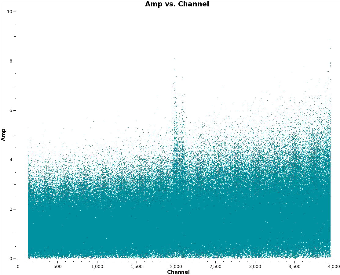 Fig. 4b: M100 7m-array Amp plotted per spw. Locate line channels to exclude from statwt.


As mentioned above in the Option 3 statwt caveats, it is essential to avoid strong line channels when calculating the statistics. At minimum, if you can see a line in a uvplot it should not be included. The easiest way to check is to make a plot of the uv-data vs channel with plotms.
# In CASA
plotms(vis='M100_Band3_12m_CalibratedData.ms',
       yaxis='amp', xaxis='channel', avgtime='1e8', avgscan=True,
       iteraxis='spw', plotfile='12m_amp_ch.png', exprange='all', overwrite=True)

plotms(vis='M100_Band3_7m_CalibratedData.ms',
       yaxis='amp', xaxis='channel', avgtime='1e8', avgscan=True,
       iteraxis='spw', plotfile='7m_amp_ch.png', exprange='all', overwrite=True)
Here we plot each spw of both data sets, and find that there are lines in 12m spw 0, and 7m spws 3,5. For this example we will adjust the weights of these spws.
- WT vs UVdist before correction
-
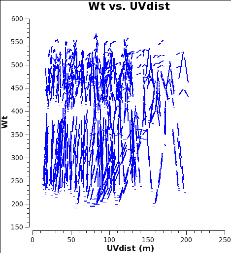 Fig. 5a: M100 12m-array weights after calibration of amplitude gains with calwt=False.
 -
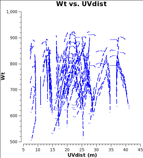 Fig. 5b: M100 7m-array weights after calibration of amplitude gains with calwt=False.


Now plot the weights before correction with plotms. No averaging can be done when plotting the weights, but you can choose a smaller channel range for speed if you like.
# In CASA
plotms(vis='M100_Band3_12m_CalibratedData.ms', spw='0', yaxis='wt', xaxis='uvdist',
       plotfile='12m_calwtF_WT.png', overwrite=True)

plotms(vis='M100_Band3_7m_CalibratedData.ms', spw='3,5', yaxis='wt', xaxis='uvdist',
       plotfile='7m_calwtF_WT.png', overwrite=True)
At this starting point, the 7m data actually have higher weight than the 12m data. This is because the average Tsys were similar but the visibility integration time of the 7m data is 10.1 versus 6.048s for the 12m data (see listobs outputs in the previous section). Imaging these data would work very poorly because as described in the previous example, the 7m should actually have weights ≈ 0.193 times lower than the 12m data.
In statwt we need to exclude the line emission channels in the fitspw parameter while sampling the full spectral range. This is especially important in this example because the CO(1-0) transition is close to an oxygen line in the atmosphere; this is what causes the noise to increase at higher channel numbers. Since we are deriving a spectrally averaged weight it would be unrealistic to only include the lower, less noisy channels.
# In CASA
statwt(vis='M100_Band3_12m_CalibratedData.ms', spw='0',
       fitspw='0:0~1700;2100~3839', datacolumn='data')

statwt(vis='M100_Band3_7m_CalibratedData.ms', spw='3,5',
       fitspw='3:0~1800;2200~4079,5:0~1800;2200~4079', datacolumn='data')

Since the correction in this example was done with statwt in CASA <=4.4, the absolute values are half of what they should be; see Option 3 in the section below.
Now we concat the data. See the listobs output in the previous example. Note that 7m spws 3,5 become spws 7,9 in the combined MS.
# In CASA
import os
os.system('rm -rf M100_Band3_statwt.ms')
concat(vis=['M100_Band3_12m_CalibratedData.ms','M100_Band3_7m_CalibratedData.ms'],
       concatvis='M100_Band3_statwt.ms')

listobs(vis='M100_Band3_statwt.ms', listfile='M100_Band3_statwt.listobs.txt')
Finally, plotms to verify that the weights have the corrected values that we expect.
# In CASA
plotms(vis='M100_Band3_statwt.ms', spw='0,7,9', yaxis='weight', xaxis='uvdist',
       coloraxis='spw', plotfile='M100_statwt_WT.png', overwrite=True)
These weights are in good agreement with those derived using the correct weights throughout calibration, as seen in M100_Band3_Combine. However, see the next section for caveats.
Absolute Accuracy of the Data Weights
As mentioned several times in this guide, good imaging performance is only subject to correct relative weights, which is achieved as of CASA >4.2.2 provided calwt=True for the amplitude gain table in applycal. Even for Case 1 (4.2.1 and lower), the relative weights within a given dataset are reasonably accurate in most cases due to the 1/Tsys2 scaling. However, there are some instances, for example, uv-model fitting where one would like to use the visibility weights as an absolute measure of 1/σ2. Here we discuss the absolute accuracy of the visibility weights for options 1 and 3:
- Option 1: All PI data taken so far with ALMA are Hanning smoothed online, but it is up to the user at proposal creation time to decide if additional channel averaging is done in the correlator (typically to reduce the data rate). Data that are Hanning smoothed but not channel averaged by the ALMA online system have a theoretical effective channel width 2.667 times that reported by for example listobs from the point of view of calculating the sensitivity of a single channel (it is a factor of 2.0 for the FWHM, i.e. channel resolution). The CASA initialization of 2ΔνchΔtij does not currently take this into account -- CASA does not have a way of knowing presently what the online system did, only how the data appears on disk, though this will change with future versions of the online software. Thus, presently CASA weights for this case are in principle a factor of 2.667 times smaller than they should be from a sensitivity point of view. For online channel averaging of two or more channels, the difference between the channel width and the effective channel width diminishes rapidly (2x channel averaging has a factor 1.6, 4x a factor 1.2, 8x a factor of 1.1). Additionally, the current weights do not include the correlator and quantization efficiencies ηq and ηc. These have values of about 0.88 and 0.96, respectively.
- ⇒ Starting in Cycle 3, the effective channel width will be recorded in the raw data and used by CASA to initialize the weights for CASA versions >=4.2.2.
- Option 3: For CASA <=4.4 statwt does not take channel-specific flagging into account, only flags that apply to all channels. Thus, the user must avoid flagged channels with the fitspw parameter. Additionally, strong line emission must be avoided. Provided these conditions are met, our tests suggest that the weights produced by statwt are too low by a factor of 2 compared to the expected values. Both of these statwt issues will be fixed as of CASA 4.5.
As a consequence, for online Hanning smoothed data with no online channel averaging, the average value of the weights resulting from Options 1 and 3 will appear to approximately match (see M100_Band3_Combine_6.6.1#Checking_the_weights_and_concatenating_the_data examples), but for erroneous reasons.
Our investigation into these matters continues so if the absolute weights are important to you, check back here or send a helpdesk ticket with your inquiry.