Simdata New Users Guide 3.1
Explanation of the guide
This guide is intended to be used as an initial walk-through of how to use simdata. We will start with an image similar to something that might be observed with ALMA, and then we will show how to rescale the image and predict how it will look when observed with different antenna configurations.
We will assume only a general knowledge of interferometry and no specific knowledge of CASA.
Getting Started
The two things you need to get started are:
- The image to work with
- The current version of CASA
To get the image, download the Spitzer IRAC 8 micron image of 30 Doradus from the Simulation Inputs CASA Guide page.
To install CASA, follow the instructions given here. This guide was written for CASA version 3.1
Using CASA
CASA is the post-processing package for ALMA and EVLA and can handle both interferometric and single dish data. Because simdata is a task within CASA, we start here with a brief introduction to some CASA basics. To learn much more about CASA, go to the CASA homepage. Walk-throughs of CASA data reduction for a variety of data sets can be found on the casaguides website.
Starting CASA
Once you have installed CASA, you can launch it by typing "casapy" at the prompt or by double-clicking on the icon, depending on your system and preferences.
Running CASA Tasks
To see a list of all available CASA tasks, at the CASA prompt type
> tasklist
To look at the inputs for an available task, use "inp". For instance
> inp simdata
Any parameter with a grey background is expandable. Red text shows an invalid value. Blue text shows an accepted, but not the default, value.
To get help on a given task, use "help". For instance
> help simdata
To reset a task to its default values, use "default". For instance
> default simdata
To run a task, just type its name at the CASA prompt. For instance
> simdata
Using Simdata
Getting Your Input Image Into Simdata

Now tell simdata where to find the model (input) image and how to scale it appropriately for our purposes. Just to be safe, we'll first restore the default values of simdata.
> default simdata
> modifymodel = True
> skymodel = '30dor.fits'
We are using a Spitzer 8 micron image of 30 Doradus in this example, and we are going to ask simdata to modify this image in some important ways:
- Angular scale
- Observed wavelength
- Brightness scale
Angular Scale
If you open the fits image of 30 Doradus in your favorite viewer, you will see that it covers quite a large footprint on the sky, about 10' on a side. We are going to tell simdata to rescale the pixels to shrink the image by roughly a factor of 15 (from 3.6" to 0.25" pixels) so that the model is approximately 40" on a side. This rescaled model will fit within a small mosaic of 6 pointings. Although we do this primarily for convenience in this example, a scientific motivation for this type of rescaling would be to approximate what a super-giant HII region like 30 Doradus would look like if moved from the Large Magellanic Cloud to the distance of M33 or M31. For the sake of demonstration, we will also change the coordinates of the center of the map.
> incell = '0.25arcsec'
> indirection = 'J2000 10h00m00 -40d00m00'
Observed Wavelength
The model image of 30 Doradus shows the 8 micron continuum emission. ALMA does not observe at wavelengths this short, so we will tell simdata that this is actually a 230 GHz (1.3 mm) continuum map. We will also tell simdata that the observations were taken with a 2 GHz bandwidth. Although for this particular example the channel width is not a critical number, it would be very important if we were modifying a spectral cube instead of a continuum image.
> incenter = '230GHz'
> inwidth = '2GHz'
Brightness Scale
The 8 micron emission is probably not a great proxy for the millimeter emission from 30 Doradus. For a true science case, one would want to calculate what the expected 230 GHz emission would be from an object like this at the distance of about 750 kiloparsec. For the sake of simplicity, we will rescale the image so that the brightest pixel in the map has a flux density of 0.1 mJy. This number is chosen such that the extended emission is a factor of a few brighter than the expected noise in a 2 hour observation.
> inbright = '0.1mJy/pixel'
Defining the Mock Observations

Now that simdata knows how to interpret the input image, the next step is to define the simulated observations.
Pointings and Scan Time
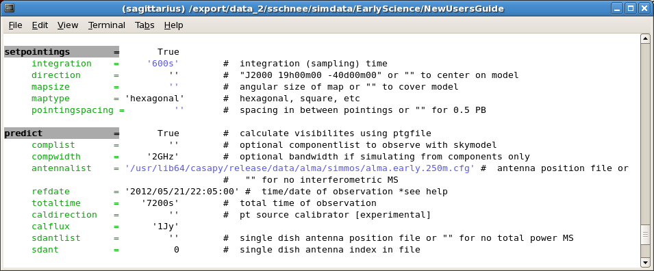
We will first change the parameters within "setpointings"
- integration
- direction
- mapsize
- maptype
- pointingspacing
The default value for "integration", 10 seconds, might be appropriate to simulate real observations. However, simdata will run much faster if the value for "integration" is increased. In this demonstration will will set it to 600 seconds. When simdata is used for scientific purposes it may be best to set "integration" to a large value at first to make sure that simdata runs as expected, and then decrease "integration" to a more realistic time for the final run.
We will keep "direction" at the default (blank) value to center the observations on the model coordinates, as given in "indirection" above.
We will set mapsize to (blank) to cover the entire model, which in our case will require a mosaic of 6 pointings (as we will see later on). The mosaic default pattern "maptype" is 'hexagonal', which we will leave unchanged.
Finally, we will change the value of "pointingspacing" to (blank) to set the pointings to be half a primary beam apart.
> integration = '600s'
> mapsize =
> pointingspacing =
Antenna Positions and Total Observation Time
Now we will consider the parameters within "predict". We will keep the default values for every parameter except "antennalist", which tells simdata the locations and sizes of each antenna in the array. We will simulate an Early Science observation, so we will first find the location where CASA has stored the ALMA configuration files. Then we will tell simdata to the the configuration file designed for Early Science.
> repodir = os.getenv("CASAPATH").split(' ')[0]
> antennalist =  repodir+"/data/alma/simmos/alma.early.250m.cfg"
The first line, run within CASA, uses a linux command to determine the path for CASA. The second line sets the "antennalist" parameter to the Early Science configuration. Other .cfg files in the same directory exist for various ALMA Full Science array configurations as well as the configuration files for other radio interferometers.
Most of the other parameters are not relevant for this simulation since we are not using a component list to describe the sky emission, we no not want to simulate observations of a calibrator, and we do not want to simulate single dish observations. Note that at this stage of development, the "refdate" parameter is ignored and all observations are instead centered around transit.
Thermal Noise
For this simple simulation, we will no include any thermal noise in the observations, so we can leave "thermalnoise" at its default (blank) value.
Choosing Simdata Output Images

Now that simdata has made the mock visibilities, it is time to invert them to make an image of sky as observed with the interferometer.
Image
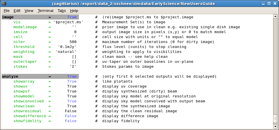
We would like to make a deconvolved output image, but we don't want to spend too much time optimizing the cleaning. So, all we need to do is set "clean" to true and leave all of the other parameters at their default values. Other data reduction guides describe the process of cleaning in greater detail.
> image = True
For simulations intended for a proposal or scientific analysis, one would want to choose a more appropriate cleaning treshold and define the region to be cleaned.
Analyze
To choose which six output images you would like simdata to create (you are limited to 6), set the parameter "analyze" to True and then pick your favorite outputs. In this example we will look at
- Locations of the antennas
- uv coverage in the 2 hour observation
- Synthesized beam (point spread function)
- Original sky model (as defined in "modifymodel"
- Convolved model (sky model convolved with the synthesized beam)
- Clean image (the sky as observed with the interferometer)
To make these choices, use the following lines in CASA
> analyze = True
> showarray = True
> showconvolved = True
> showdifference = False
> showfidelity = False
Final Check
Finally, check that everything looks correct. Look at the simdata inputs and compare with the screen shots shown above. You may want to change "overwrite" to True so that future runs with slightly changed parameters don't crash.
> overwrite = True
> inp simdata
If everything looks promising, then run simdata.
> simdata
Simdata Output Images
Simdata will display output images to your screen, partly based on your selections in "analyze". It will also produce images that you can display for yourself using the viewer tool that comes with CASA.
Figures Plotted to the Screen
When simdata is run with the parameters set as above, the images plotted to the screen are:
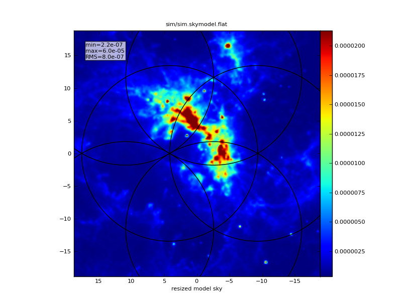
- The model image, rescaled as defined in "modifymodel", with the mosaic pointings as defined in "setpointings"

Input (sky model) image with mosaic pointings overlayed - Plots related to "predict", with
- Source elevation vs. time
- The positions of the antennas
- The uv coverage
- The synthesized beam (psf)
- Images of the 30 Doradus
- The original image, as defined in "modifymodel"
- The original image convolved with the psf
- The "observed" image
- The difference the observed and original image
- The images requested in "analyze"

Plots requested in "analyze" - The antenna plot
- The uv coverage
- The synthesized beam
- The sky model image
- The convolved sky model
- The "observed" image
If the images don't stay on your screen long enough to analyze, you can make simdata save the images as .png files with the "graphics" parameter.
> graphics = 'file'
Using Viewer
thumb|Simdata-generated images that can be loaded with the CASA viewer
Simdata also creates several images that can be displayed with the CASA viewer tool. The viewer can be launched within CASA by typing
> viewer
You will be shown several files that you can view, including those made by CASA and the original FITS image. Some of the more important images are:
- sim.image - The simulated observations
- sim.image.flat - The moment 0 map of the simulated observations (for continuum observations like those in this example, this is not relevant)
- sim.skymodel - The input map/cube as defined in "modifymodel"
- sim.psf - The synthesized beam
- sim.residual - The difference between the sky model and the simulated observations
You can learn a lot about the functionality of the CASA viewer by watching this instructional video.