IRAS16293 Band9 - Calibration for CASA 6.4
- This guide is written for CASA 6.4.1.12 and uses Python 3.6.
- This script assumes that you have downloaded IRAS16293_Band9_UnCalibratedMS.tgz from IRAS16293Band9#Obtaining the Data.
- Details of the ALMA observations are provided at IRAS16293Band9.
- This portion of the guide covers calibration of the raw visibility data. To skip to the imaging portion of the guide, see: IRAS16293 Band9 - Imaging for CASA 6.4.
WARNING: On June 15, 2012 the calibration guide and the final data products (calibrated science
data: IRAS16293_Band9_CalibratedMS_FIXED.tgz and reference images: IRAS16293_Band9_ReferenceImages_FIXED.tgz))
were changed to correct for a 1.2" position error in the phase calibrator (1625-254). Without
correction, the science images will suffer from a similar offset.
Overview
This part of the casa guide will guide you through the basic inspection of the data, paying special attention to identifying data that needs to be flagged. The guide shows the complete process to get fully calibrated data.
The general procedure in this guide follows the other ALMA CASA guides: NGC3256Band3 and AntennaeBand7.
Unpack the Data
Make sure you have downloaded the data from IRAS16293Band9#Obtaining_the_Data.
Once you have downloaded the IRAS16293_Band9_UnCalibratedMS.tgz, unpack the file in a terminal outside CASA using
# in bash

tar -xvzf IRAS16293_Band9_UnCalibratedMS.tgz

cd IRAS16293_Band9_UnCalibratedMS
You have a number of files with extensions ".ms", which are CASA measurement set (MS) files. Within each MS file you will also see files containing system temperature (Tsys), water vapor radiometer (WVR), and antenna position information.
To start CASA type
# in bash
casa
Be sure that you are using the right version indicated for this guide.
Confirm your version of CASA
This guide has been written for CASA release 6.4.1.12. Please confirm your version before proceeding. You can find guides written for previous CASA versions at IRAS16293Band9#IRAS16293_Band_9_Data_Reduction_Tutorial.
# In CASA
import casalith
version = casalith.version_string()
print ("You are using " + version)
if (version < '6.4.1.12'):
    print ("YOUR VERSION OF CASA IS TOO OLD FOR THIS GUIDE.")
    print ("PLEASE UPDATE IT BEFORE PROCEEDING.")
else:
    print ("Your version of CASA is appropriate for this guide.")
Install Analysis Utilities
Analysis Utilities (or analysisUtils for short) is a small set of Python scripts that provide a number of analysis and plotting utilities for ALMA data reduction. This guide uses a few of these utilities. They are very easy to install (just download and untar). See
http://casaguides.nrao.edu/index.php?title=Analysis_Utilities
for a full description and download instructions. If you do not wish to do this, see a CASA 3.3 version of one of the other ALMA guides for alternative (but slow) plotting options. Analysis Utilities are updated frequently so if its been a while since you installed it, it's probably worth doing it again. If you are at an ALMA site or ARC, the analysis utilities are probably already installed and up to date.
Initial Inspection
The first step we will go through all the calibration process is to define an array with the uid's that correspond to the dataset names. This will allow us to make the calibration of the four datasets one after another, using a for-loop inside python. We will then calibrate the data individually and concatenate them at the end, before proceeding with the imaging part.
Note that if you exit CASA and want to continue with the calibration using these arrays, you will have to re-issue the command again to make it available for the current CASA execution.
To start, and give an example of this process, we will create txt format files for the output of the listobs task, which will give us useful information about the observations.
# In CASA
# Array containing the uid names

rawdata=['uid___A002_X3d4118_X39b.ms','uid___A002_X3d55cb_X575.ms',
         'uid___A002_X3d55cb_Xb50.ms','uid___A002_X3d55cb_X90c.ms']

# We create the text files for listobs for each dataset

for data in rawdata:
  listobs(vis=data,listfile=data+'.listobs')
Note that after cutting and pasting a for-loop you often have to press return several times to make the command execute. The output will be sent to text files with the extension *.listobs. Next, we show an example of a useful part of the output that the first listobs command (from execution X39b) produces.
Fields: 11
  ID   Code Name                RA               Decl           Epoch   SrcId      nRows
  0    none 1924-292            19:24:51.056000 -29.14.30.12800 J2000   0         169125
  1    none nrao530 ph          17:33:02.724000 -13.04.49.48600 J2000   1         289170
  2    none Juno                16:25:31.630312 -05.49.08.92088 J2000   2          82890
  3    none 1625-254            16:25:46.980000 -25.27.38.33000 J2000   3         276480
  4    none IRAS16293-2422-a    16:32:22.992000 -24.28.36.00000 J2000   4         132450
  5    none IRAS16293-2422-a    16:32:22.479253 -24.28.36.00000 J2000   4          99915
  6    none IRAS16293-2422-a    16:32:22.735626 -24.28.36.00000 J2000   4          99960
  7    none IRAS16293-2422-a    16:32:22.735626 -24.28.32.50000 J2000   4          99915
  8    none IRAS16293-2422-a    16:32:22.479253 -24.28.29.00000 J2000   4          99945
  9    none IRAS16293-2422-a    16:32:22.735626 -24.28.29.00000 J2000   4          99945
  10   none IRAS16293-2422-a    16:32:22.992000 -24.28.29.00000 J2000   4          99915
Spectral Windows:  (25 unique spectral windows and 2 unique polarization setups)
  SpwID  Name                           #Chans   Frame   Ch0(MHz)  ChanWid(kHz)  TotBW(kHz) CtrFreq(MHz) BBC Num  Corrs
  0      WVR#NOMINAL                         4   TOPO  184550.000   1500000.000   7500000.0 187550.0000        0   I
  1      ALMA_RB_06#BB_1#SW-01#FULL_RES    128   TOPO  231257.813     15625.000   2000000.0 232250.0000        1  XX  YY
  2      ALMA_RB_06#BB_1#SW-01#CH_AVG        1   TOPO  232234.375   1796875.000   1796875.0 232234.3750        1  XX  YY
  3      ALMA_RB_06#BB_2#SW-01#FULL_RES    128   TOPO  229257.813     15625.000   2000000.0 230250.0000        2  XX  YY
  4      ALMA_RB_06#BB_2#SW-01#CH_AVG        1   TOPO  230234.375   1796875.000   1796875.0 230234.3750        2  XX  YY
  5      ALMA_RB_06#BB_3#SW-01#FULL_RES    128   TOPO  217242.188    -15625.000   2000000.0 216250.0000        3  XX  YY
  6      ALMA_RB_06#BB_3#SW-01#CH_AVG        1   TOPO  216234.375   1796875.000   1796875.0 216234.3750        3  XX  YY
  7      ALMA_RB_06#BB_4#SW-01#FULL_RES    128   TOPO  215242.188    -15625.000   2000000.0 214250.0000        4  XX  YY
  8      ALMA_RB_06#BB_4#SW-01#CH_AVG        1   TOPO  214234.375   1796875.000   1796875.0 214234.3750        4  XX  YY
  9      ALMA_RB_09#BB_1#SW-01#FULL_RES    128   TOPO  703257.813     15625.000   2000000.0 704250.0000        1  XX  YY
  10     ALMA_RB_09#BB_1#SW-01#CH_AVG        1   TOPO  704234.375   1796875.000   1796875.0 704234.3750        1  XX  YY
  11     ALMA_RB_09#BB_2#SW-01#FULL_RES    128   TOPO  692492.188    -15625.000   2000000.0 691500.0000        2  XX  YY
  12     ALMA_RB_09#BB_2#SW-01#CH_AVG        1   TOPO  691484.375   1796875.000   1796875.0 691484.3750        2  XX  YY
  13     ALMA_RB_09#BB_3#SW-01#FULL_RES    128   TOPO  690492.188    -15625.000   2000000.0 689500.0000        3  XX  YY
  14     ALMA_RB_09#BB_3#SW-01#CH_AVG        1   TOPO  689484.375   1796875.000   1796875.0 689484.3750        3  XX  YY
  15     ALMA_RB_09#BB_4#SW-01#FULL_RES    128   TOPO  688492.188    -15625.000   2000000.0 687500.0000        4  XX  YY
  16     ALMA_RB_09#BB_4#SW-01#CH_AVG        1   TOPO  687484.375   1796875.000   1796875.0 687484.3750        4  XX  YY
  17     ALMA_RB_09#BB_1#SW-01#FULL_RES   3840   TOPO  703312.744       488.281   1875000.0 704250.0000        1  XX  YY
  18     ALMA_RB_09#BB_1#SW-01#CH_AVG        1   TOPO  704249.756   1875000.000   1875000.0 704249.7559        1  XX  YY
  19     ALMA_RB_09#BB_2#SW-01#FULL_RES   3840   TOPO  692237.256      -488.281   1875000.0 691300.0000        2  XX  YY
  20     ALMA_RB_09#BB_2#SW-01#CH_AVG        1   TOPO  691299.756   1875000.000   1875000.0 691299.7559        2  XX  YY
  21     ALMA_RB_09#BB_3#SW-01#FULL_RES   3840   TOPO  690437.256      -488.281   1875000.0 689500.0000        3  XX  YY
  22     ALMA_RB_09#BB_3#SW-01#CH_AVG        1   TOPO  689499.756   1875000.000   1875000.0 689499.7559        3  XX  YY
  23     ALMA_RB_09#BB_4#SW-01#FULL_RES   3840   TOPO  688437.256      -488.281   1875000.0 687500.0000        4  XX  YY
  24     ALMA_RB_09#BB_4#SW-01#CH_AVG        1   TOPO  687499.756   1875000.000   1875000.0 687499.7559        4  XX  YY

Antennas: 15:
  ID   Name  Station   Diam.    Long.         Lat.                Offset from array center (m)                ITRF Geocentric coordinates (m)
                                                                     East         North     Elevation               x               y               z
  0    DA41  A003      12.0 m   -067.45.16.5  -22.53.27.0         35.5311     -672.6372       21.8405  2225083.646015 -5440070.406024 -2481658.026558
  1    DA43  A075      12.0 m   -067.45.17.9  -22.53.21.4         -4.5601     -499.7013       23.0314  2225072.420395 -5440148.857922 -2481499.171513
  2    DA47  A026      12.0 m   -067.45.18.8  -22.53.28.3        -28.8060     -712.8991       22.1464  2225018.277767 -5440080.526423 -2481695.236840
  3    DV02  A077      12.0 m   -067.45.10.1  -22.53.25.9        217.6305     -637.5330       15.8360  2225255.259378 -5440008.986376 -2481623.351197
  4    DV03  A137      12.0 m   -067.45.15.2  -22.53.22.7         71.1264     -540.4366       20.6163  2225135.630926 -5440103.481566 -2481535.759910
  5    DV05  A082      12.0 m   -067.45.08.3  -22.53.29.2        269.0429     -740.9517       15.7820  2225287.593084 -5439952.242959 -2481718.604490
  6    DV07  A076      12.0 m   -067.45.20.5  -22.53.33.8        -77.9902     -882.7193       24.0686  2224948.419151 -5440039.640642 -2481852.430221
  7    DV09  A046      12.0 m   -067.45.17.0  -22.53.29.3         21.4254     -742.7980       21.1731  2225060.026237 -5440049.916625 -2481722.402511
  8    DV10  A071      12.0 m   -067.45.19.9  -22.53.23.5        -60.7886     -563.2541       23.3802  2225011.142129 -5440147.561183 -2481557.855799
  9    DV12  A011      12.0 m   -067.45.14.4  -22.53.28.4         95.9123     -716.4998       21.0909  2225132.809916 -5440031.116953 -2481698.143375
  10   DV13  A072      12.0 m   -067.45.12.6  -22.53.24.0        147.1743     -580.5886       18.1818  2225199.254234 -5440058.160957 -2481571.803351
  11   DV14  A025      12.0 m   -067.45.18.7  -22.53.27.4        -26.4285     -685.5220       21.7070  2225024.356358 -5440089.108350 -2481669.844738
  12   DV15  A074      12.0 m   -067.45.12.1  -22.53.32.0        161.8155     -828.6194       18.7683  2225176.483017 -5439963.820241 -2481800.529472
  13   DV17  A138      12.0 m   -067.45.17.1  -22.53.34.4         19.1458     -901.2602       26.0146  2225036.269071 -5439997.854035 -2481870.267809
  14   DV18  A053      12.0 m   -067.45.17.3  -22.53.31.2         12.5950     -802.9951       21.5079  2225043.105532 -5440031.871503 -2481777.989003
In the previous output you can see the ID that is assigned to each source, starting with the number 0. Examine the listobs files for each of the four executions. 1924-292 and 3c279 are the calibrators for bandpass, Juno for amplitude (flux), 1625-254 is our phase calibrator and nrao530 ph serves as a check (phase calibrator) source. The remaining 7 fields of IRAS16293-2422-a are the seven pointings for our mosaic of the target source. Notice that in the example above 1924-292 is the bandpass calibrator. Other executions use 3c279 as a bandpass calibrator.
Spectral windows are also marked with numbers from 0 to 24, with number 0 containing WVR information. Spws 17, 19, 21, and 23 contain the science data (FDM mode). The CO (6-5) line emission is contained in spw 19. Spw 18, 20, 22, and 24 contain channel averages of the data from spectral windows 17, 19, 21, 23, respectively. These spws will not be used for the offline data reduction. All the remaining spws that appear in the section of "Sources", and that do not appear in the "Spectral Windows" section are related to water vapor radiometer (WVR) measurements for each antenna, so you will not need them for the calibration either. Spws 9, 11, 13, and 15 are associated with tsys measurements, and we will apply these measurements to the science spws later.
Finally before we go further we explicitly save the current flag state of the data.
# In CASA
# Use flagmanager to save current flag state.

for vis in rawdata:
  flagmanager(vis=vis,mode='save',versionname='OriginalFlagState')
If you ever decide to start completely over, you should substitute 'restore' for 'save' in the command below to restore the flag state to its original value.
Generation and visualization of the antenna positions, Tsys and WVR tables
Next we will generate the tables we need to apply to the data: antenna position, system temperature (tsys) and water vapor radiometer (WVR). Once the tables are generated we will produce plots of them and inspect them to make sure whether they have issues that might affect their application to the data. Whenever we see an odd behavior in the tables we need to flag the corresponding science data to prevent wrong results in the calibration steps.
System Temperature
We produce the Tsys tables with the next command. Note that you will see warnings reporting that some spw are completely flagged. This is expected.
# In CASA
# Array containing the uid names
rawdata=['uid___A002_X3d4118_X39b.ms','uid___A002_X3d55cb_X575.ms',
         'uid___A002_X3d55cb_Xb50.ms','uid___A002_X3d55cb_X90c.ms']

# Create Tsys
os.system('rm -rf *tdm.tsys')
for vis in rawdata:
    print ("Creating TDM Tsys Table for "+vis)
    gencal(vis=vis,caltable=vis+'.tdm.tsys',spw='9,11,13,15',caltype='tsys')
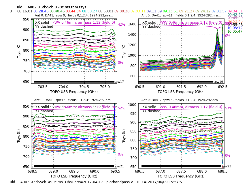
The next command will plot the tsys in the next way: it will produce many plots, each one of them will show an antenna, with the four spws that the tsys tables cover, for all the targets, and with different colors for different times, so you can trace the behavior for tsys with time, among others. Note that in spw 19, the overlap with the tsys spw (11) is not set correctly. This is due to an error in the frequencies for the tsys when the observations were done. You do not have to worry about this, since any issue coming from that error has already been fixed. Note, however that the portions of the spectra that do not have tsys information cannot be used. This does not represent a problem, since that part corresponds to the edge of the baseband. Also note that the CO (6-5) line is not affected by this. You will see warnings that all data for Juno is flagged. This is expected and not an issue as it is accounted for in later commands. In Figure 1 you will see the corresponding plot for one of the datasets (X90c) showing antenna 0 (DA41).
# In CASA
# Plot TDM Tsys tables with times overlayed for each antenna
os.system('rm -rf Tsysplots/*time*')
for vis in rawdata:
  plotbandpass(caltable=vis+'.tdm.tsys',vis=vis,
                overlay='time', xaxis='freq', showatm=True,
                yaxis='amp',subplot=22,interactive=False,
                chanrange='5~122',showfdm=True,
                figfile='Tsysplots/'+vis+'.time.tdm.tsys.png')
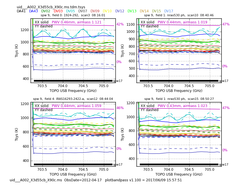
Another useful set of plots is generated by the next command. Each resulting plot shows all the antennas in a scan, for one spectral windows. This is useful to check Tsys for all the antennas in a certain time. In Figure 2 you can see an example. You may safely ignore the multiple warnings about "Adding an axes using the same arguments as a previous axes..." The warning is just referring to a deprecated feature in the plotting library used by the plotbandpass command.
# In CASA
# Plot TDM Tsys tables with antennas overlayed for each time
os.system('rm -rf Tsysplots/*antenna*')
for vis in rawdata:
  plotbandpass(caltable=vis+'.tdm.tsys',vis=vis,
                overlay='antenna', xaxis='freq', showatm=True,
                yaxis='amp',subplot=22,interactive=False,
                chanrange='5~122',showfdm=True,
                figfile='Tsysplots/'+vis+'.antenna.tdm.tsys.png')
The plots will be put into the Tsysplots directory. Go through all the plots and make sure you notice all of the issues listed below, since we will need to flag the corresponding science data. You should notice a spike in tsys on the edge of tsys spw 11. This is due to a slight decrease in atmospheric transmission at this frequency and is expected. The magenta line at the top of each plot shows the atmospheric transparency and the percentage transmission is labelled. We have noted the range of tsys and atmospheric transmission levels for each execution below. These values exclude the outliers that are noted. Specific spws refer to the science spw. Although the tsys is measured in a different spw, we will ultimately end up flagging the affected science spw. Therefore, we note outliers based on the science spw.
 X90c
 DV05 shows ripples in all spw
 Otherwise 600 to 1200; 47 to 57% transmission

 X575
 Otherwise 1300 to 3000; 28 to 39% transmission
 DV05 shows ripples in all spw
 DV10 ripples in YY in spws 21 and 23

 Xb50
 800 to 2500; 37 to 47% transmission
 DV05 shows ripples in all spw

 X39b
 500 to 800; 56 to 65%
 DA43 Tsys extremely high for spw=23
 DV03 shows ripples in spw 23 in YY
 DV05 shows ripples in all spw and one time with bad YY
 DV18 extremely high for spw=23
Water Vapor Radiometer (WVR)
We now generate the WVR tables by executing wvrcal. For more information on the WVR measurement and application, see the ALMA Technical Handbook. Note that here we use a toffset (time offset) = -1. This was the default for ALMA up to January 2013. Later ALMA data uses a time offset between the interfermetric and WVR data of 0 seconds, which is the default in current CASA versions.
# In CASA
rawdata=['uid___A002_X3d4118_X39b.ms','uid___A002_X3d55cb_X575.ms',
         'uid___A002_X3d55cb_Xb50.ms','uid___A002_X3d55cb_X90c.ms']

# Other values can be left at defaults
os.system('rm -rf *.wvrgcal')
for vis in rawdata:
    wvrgcal(vis=vis,caltable=vis+'.wvr',toffset=-1)
The integration time for the science spectral windows is 6.048 seconds. So we need to average the WVR 1 second solutions to match. The smoothing avoids the introduction of additional phase noise.
# In CASA
# Smoothing the data
for vis in rawdata:
  print ("Smoothing wvr table for  "+vis)
  smoothcal(vis=vis,tablein=vis+'.wvr',caltable=vis+'.wvr.smooth',
            smoothtype='mean',smoothtime=6.048)
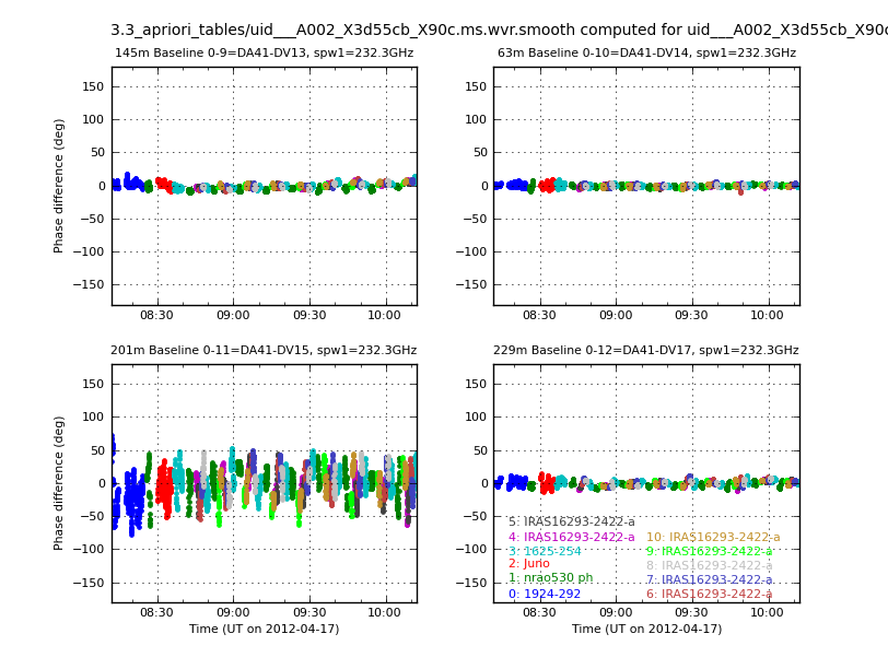
Now, for the plotting of the wvr tables, we will employ the Analysis utils package. This command will create a directory called WVRplots with all the plots inside, each one of them corresponding to different datasets, baselines and targets, using different colors. In Figure 3 you can see an example of the output for spectral window 1. Note that the command below only creates the plots for that spw, since the others are the same except for a scale factor that is the ratio of frequencies. Note that in all datasets, DV15 has bad wvr behavior.
# In CASA
# Plotting wvr tables for spw 1
os.system('rm -rf WVRplots')
for vis in rawdata:
  au.plotWVRSolutions(caltable=vis+'.wvr.smooth',
              yrange=[-180,180],figfile='WVRplots/'+vis+'.wvr.smooth.png',
              ms=vis,spw='1',interactive=False)
Antenna position
Finally, we need to create the tables to correct for the antenna positions. These are small corrections to the position of each antenna based on regularly run calibration observations. For that, execute
# In CASA
# Generate the tables for antenna positions
rawdata=['uid___A002_X3d4118_X39b.ms','uid___A002_X3d55cb_X575.ms',
         'uid___A002_X3d55cb_Xb50.ms','uid___A002_X3d55cb_X90c.ms']

# For the data taken on April 16
antennas='DV18,DV12,DV09,DV10,DV13,DV05,DA41,DV14,DA43,DV17,DV07,DV15'
parameter=[0.00684754783288,-0.0188271608204,-0.00732900947332,
0.000481227821554,-2.48519197708e-05,-0.00048066949752,
0.000741523189806,-0.000843518709779,-0.000409113120338,
0.00111751207514,-0.000891124202747,-0.000492116263895,
0.00100313175518,-0.00084909900337,-0.000594194887412,
0.00105206234994,-0.000857719516042,-0.00059565765641,
0.00060776527971,-0.000525096431375,-0.000386487226933,
0.000521688542419,-0.000144920371688,-0.000258341151538,
0.00104740676978,-0.000899314162014,-0.000483014592547,
0.000920921096116,-0.00106288533016,-0.000546355296173,
0.000867350985729,-0.000990079062422,-0.00038123971161,
0.000567245762795,-0.000422531738877,-0.000741700641811]
gencal(vis = 'uid___A002_X3d4118_X39b.ms',
  caltable = 'uid___A002_X3d4118_X39b.ms.antpos',
  caltype = 'antpos',antenna=antennas,parameter=parameter)

# and for April 17
antennas='DV05,DV09,DV10,DV13,DV12,DA41,DV14,DA43,DV17,DV07,DV15'
parameter=[0.00105206234994,-0.000857719516042,-0.00059565765641,
0.000741523189806,-0.000843518709779,-0.000409113120338,
0.00111751207514,-0.000891124202747,-0.000492116263895,
0.00100313175518,-0.00084909900337,-0.000594194887412,
0.000481227821554,-2.48519197708e-05,-0.00048066949752,
0.00060776527971,-0.000525096431375,-0.000386487226933,
0.000521688542419,-0.000144920371688,-0.000258341151538,
0.00104740676978,-0.000899314162014,-0.000483014592547,
0.000920921096116,-0.00106288533016,-0.000546355296173,
0.000867350985729,-0.000990079062422,-0.00038123971161,
0.000567245762795,-0.000422531738877,-0.000741700641811]
for vis in range(1,4):
  gencal(vis=rawdata[vis],
    caltable=rawdata[vis]+'.antpos',
    caltype ='antpos',antenna=antennas,parameter=parameter)
These values are found by querying an observatory database. This database is not user accessible. All ALMA calibrations will include these corrections if necessary. Contact the ALMA Helpdesk if you have questions about antenna position corrections for your specific data.
Flag Data
Now, based on the behavior of the tsys and wvr tables, we will flag the corresponding data, using the next commands. You can employ similar executions to flag other data you might want to remove.
# In CASA
rawdata=['uid___A002_X3d4118_X39b.ms','uid___A002_X3d55cb_X575.ms',
         'uid___A002_X3d55cb_Xb50.ms','uid___A002_X3d55cb_X90c.ms']


# Flagging corresponding science data for tsys and wvr showing problems
for vis in rawdata:
  flagdata(vis=vis,autocorr = True,flagbackup = False)
  flagdata(vis=vis,mode='shadow',flagbackup=False)
  flagdata(vis=vis,antenna='DV05,DV15',flagbackup=False)

vis='uid___A002_X3d55cb_X575.ms'
flagdata(vis=vis,antenna='DV10',spw='21,23',flagbackup=False)

vis='uid___A002_X3d4118_X39b.ms'
flagdata(vis=vis,antenna='DA43,DV18',spw='23',flagbackup=False)
flagdata(vis=vis,antenna='DV03',spw='17',flagbackup=False)
Applying antpos, tsys, and wvr tables and splitting the data
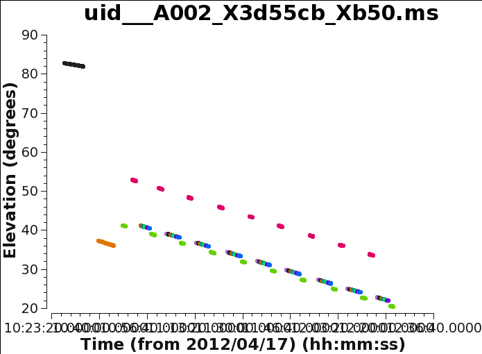
Next we will apply the tsys tables. However, not all fields have tsys measurements. IRAS16293 field (id=4) is the only target field with tsys measurements. As you probably noted from the messages from plotbandpass, the tsys measurements on Juno did not yield usable values. For fields lacking tsys measurements, we need to apply the nearest source in elevation to it. This can be checked with the plots generated by the following plotms commands. In Figure 4 you can see the output of this command for Xb50. For both cases, the nearest field with tsys measurements in IRAS16293 field id=4.
# In CASA
# Re-entering our array
rawdata=['uid___A002_X3d4118_X39b.ms','uid___A002_X3d55cb_X575.ms',
         'uid___A002_X3d55cb_Xb50.ms','uid___A002_X3d55cb_X90c.ms']

# Elevation plots to understand what the elevation range for each dataset is.
for vis in rawdata:
  plotms(vis=vis,
       field='',xaxis='time', yaxis='elevation',antenna='',
       spw='17', avgchannel='3840',coloraxis='field', showgui=True,
       ydatacolumn='data',plotfile=vis+'elevation.png',title=vis)
To apply the Tsys we need to explicitly tell applycal which TDM (128 channels) spws go with which FDM spw (3840 channels). Remember that in this case, the TDM windows are the tsys spws and the FDM windows are the science spws. An entry is needed for every spw, because the position in the list corresponds to the spw id to be corrected. There is a helper function to assist you in figuring this out.
# In CASA
from casarecipes.almahelpers import tsysspwmap
tsysspwmap(vis='uid___A002_X3d4118_X39b.ms',
           tsystable='uid___A002_X3d4118_X39b.ms.tdm.tsys')

# This will print:
# [0,1,2,3,4,5,6,7,8,9,9,11,11,13,13,15,15,9,9,19,20,13,13,15,15,25,26,27,28,29,30,31,32,33,34,35,36,37,38]
The helper gets a little confused in this case with spws 19 and 20 because the FDM was not perfectly positioned within the TDM window as you can see from the Tsys plots. In a case like this, we need to put in by hand the TDM window that should match the FDM window.
As you could see from the first run of listobs, 1924-292 is the bandpass calibrator for three of the datasets, and 3c279 is for one of them. For this reason, the application of the tables is split into two parts.
For the applycal task, note that the first value in the interp parameter for each gaintable gives the desired time interpolation type. The second parameter indicates the desired frequency axis interpolation. If the second value is not set it is assumed to be linear, but only if the input table has a frequency axis (like Tsys and Bandpass). Spline seems to work best for the Tsys TDM to FDM frequency interpolation.
# In CASA
rawdata=['uid___A002_X3d4118_X39b.ms','uid___A002_X3d55cb_X575.ms',
         'uid___A002_X3d55cb_Xb50.ms','uid___A002_X3d55cb_X90c.ms']

tsysspw=[0,1,2,3,4,5,6,7,8,9,9,11,11,13,13,15,15,9,9,11,11,13,13,15,15]

# Datasets with 1924-292 as the bandpass calibrator
for vis in [rawdata[0],rawdata[2],rawdata[3]]:
  print ("Applying calibration for "+vis)
  field_Tsys=['1924-292','nrao530 ph']
  for field in field_Tsys:
    print ("For Field= "+field)
    applycal(vis=vis,field=field,
             spw = '17,19,21,23',
             gaintable = [vis+'.tdm.tsys',
                          vis+'.wvr.smooth',
                          vis+'.antpos'],
             gainfield = [field,field,''],
             spwmap=[tsysspw,[],[]],
             interp = ['linear,spline','nearest',''],calwt = True,
             flagbackup = False)


# This next applycal takes care of the fact that one dataset has 3C279
# instead of 1924-292 as the bandpass calibrator

for vis in [rawdata[1]]:
  print ("Applying calibration for "+vis)
  field_Tsys=['3c279','nrao530 ph']
  for field in field_Tsys:
    print ("For Field= "+field)
    applycal(vis=vis,field=field,
             spw = '17,19,21,23',
             gaintable = [vis+'.tdm.tsys',
                          vis+'.wvr.smooth',
                          vis+'.antpos'],
             gainfield = [field,field,''],
             spwmap=[tsysspw,[],[]],
             interp = ['linear,spline','nearest',''],calwt = True,
             flagbackup = False)

# Next we do the "noTsys" sources for all datasets

for vis in rawdata:
  print ("Applying calibration for "+vis)
  field_noTsys=['Juno','1625-254','IRAS16293*']
  for field in field_noTsys:
    print ("For Field= "+field)
    applycal(vis =vis,field=field,
             spw = '17,19,21,23',
             gaintable = [vis+'.tdm.tsys',
                          vis+'.wvr.smooth',
                          vis+'.antpos'],
             gainfield = ['4',field,''],
             spwmap=[tsysspw,[],[]],
             interp = ['linear,spline','nearest',''],calwt = True,
             flagbackup = False)
Now that the wvr, tsys, and antenna position corrections have been applied, we only need to work with the science spws for the rest of the calibration. We will split this data with the applied calibrations to keep the measurement sets smaller and easier to work with. This may take a while, so be patient!
# In CASA
# Splitting the science spws

for vis in rawdata:
  split(vis=vis,outputvis=('%s.antwvrtsys.ms'%(vis.split('.')[0])),
        datacolumn='corrected',spw='17,19,21,23',keepflags=False)
Fix Phase Calibrator Position
The position used for the phase calibrator (1625-254) in these observations is offset by about 1.2" toward postive R.A from its correct position. Below we correct the data for this offset. It is best to do this step before doing any of the gain calibration. It is notable that simply shifting the images for this offset will not give as correct a result due to phase delays caused by sky rotation during the course of each observation.
# In CASA
data=['uid___A002_X3d4118_X39b.antwvrtsys.ms',
      'uid___A002_X3d55cb_X575.antwvrtsys.ms',
      'uid___A002_X3d55cb_X90c.antwvrtsys.ms',
      'uid___A002_X3d55cb_Xb50.antwvrtsys.ms']
List the data to see current position of 1625-254
# In CASA
for vis in data:
  listobs(vis=vis,listfile=vis+'.listobs',verbose=True)
Incorrect position from listobs: 1625-254 16h25m46.891639s -25d27m38.236880s J2000
From the EVLA calibrator manual, we find that the correct position is: 16h25m46.891639s -25d27m38.326880s J2000
Next use the task fixvis to correct the position of the calibrator in the data and the header. It will also recalculate UVWs, but this correction is very small for a 1.2" shift. Note that in more recent versions of CASA, fixvis is deprecated and is now Template:Phaseshift.
# In CASA
for vis in data:
  fixvis(vis=vis,outputvis=vis+'.fixed',field='1625-254',reuse=False,
         phasecenter='J2000 16h25m46.891639s -25d27m38.326880s',
         datacolumn='DATA')
Data inspection
We now need to check for any bad behavior in the data through several plots. Once problems are identified, data can be flagged. But before that, we need to run again listobs to check that the split and calibrator position correction worked as expected. We will define our new array of split and corrected datasets.
# In CASA
# New array of datasets
data=['uid___A002_X3d4118_X39b.antwvrtsys.ms.fixed',
      'uid___A002_X3d55cb_X575.antwvrtsys.ms.fixed',
      'uid___A002_X3d55cb_X90c.antwvrtsys.ms.fixed',
      'uid___A002_X3d55cb_Xb50.antwvrtsys.ms.fixed']

for vis in data:
    listobs(vis=vis,listfile=vis+'.listobs',verbose=True)
You can explore any of the output files by doing cat file.listobs or using any other text reader from a terminal not running CASA. Next you can see the output for X90c, and you will see the change in the spw naming, among others.
Fields: 11
  ID   Code Name                RA               Decl           Epoch   SrcId      nRows
  0    none 1924-292            19:24:51.056000 -29.14.30.12800 J2000   0          11000
  1    none nrao530 ph          17:33:02.724000 -13.04.49.48600 J2000   1          19800
  2    none Juno                16:25:05.611696 -05.43.27.92103 J2000   2           8800
  3    none 1625-254            16:25:46.891639 -25.27.38.32688 J2000   3          22000
  4    none IRAS16293-2422-a    16:32:22.992000 -24.28.36.00000 J2000   4           9900
  5    none IRAS16293-2422-a    16:32:22.479253 -24.28.36.00000 J2000   4           9900
  6    none IRAS16293-2422-a    16:32:22.735626 -24.28.36.00000 J2000   4           9900
  7    none IRAS16293-2422-a    16:32:22.735626 -24.28.32.50000 J2000   4           9900
  8    none IRAS16293-2422-a    16:32:22.479253 -24.28.29.00000 J2000   4           8800
  9    none IRAS16293-2422-a    16:32:22.735626 -24.28.29.00000 J2000   4           8800
  10   none IRAS16293-2422-a    16:32:22.992000 -24.28.29.00000 J2000   4           8800
Spectral Windows:  (4 unique spectral windows and 1 unique polarization setups)
  SpwID  Name                           #Chans   Frame   Ch0(MHz)  ChanWid(kHz)  TotBW(kHz) CtrFreq(MHz) BBC Num  Corrs
  0      ALMA_RB_09#BB_1#SW-01#FULL_RES   3840   TOPO  703312.744       488.281   1875000.0 704250.0000        1  XX  YY
  1      ALMA_RB_09#BB_2#SW-01#FULL_RES   3840   TOPO  692237.256      -488.281   1875000.0 691300.0000        2  XX  YY
  2      ALMA_RB_09#BB_3#SW-01#FULL_RES   3840   TOPO  690437.256      -488.281   1875000.0 689500.0000        3  XX  YY
  3      ALMA_RB_09#BB_4#SW-01#FULL_RES   3840   TOPO  688437.256      -488.281   1875000.0 687500.0000        4  XX  YY
         Sources: 20
  ID   Name                SpwId RestFreq(MHz)  SysVel(km/s)
  0    1924-292            0     -              -
  0    1924-292            1     -              -
  0    1924-292            2     -              -
  0    1924-292            3     -              -
  1    Juno                0     -              -
  1    Juno                1     -              -
  1    Juno                2     -              -
  1    Juno                3     -              -
  2    1625-254            0     -              -
  2    1625-254            1     -              -
  2    1625-254            2     -              -
  2    1625-254            3     -              -
  3    nrao530 ph          0     -              -
  3    nrao530 ph          1     -              -
  3    nrao530 ph          2     -              -
  3    nrao530 ph          3     -              -
  4    IRAS16293-2422-a    0     -              -
  4    IRAS16293-2422-a    1     -              -
  4    IRAS16293-2422-a    2     -              -
  4    IRAS16293-2422-a    3     -              -
Antennas: 11:
  ID   Name  Station   Diam.    Long.         Lat.                Offset from array center (m)                ITRF Geocentric coordinates (m)
                                                                     East         North     Elevation               x               y               z
  0    DA41  A003      12.0 m   -067.45.16.5  -22.53.27.0         35.5311     -672.6372       21.8405  2225083.646015 -5440070.406024 -2481658.026558
  1    DA43  A075      12.0 m   -067.45.17.9  -22.53.21.4         -4.5601     -499.7013       23.0314  2225072.420395 -5440148.857922 -2481499.171513
  2    DV02  A077      12.0 m   -067.45.10.1  -22.53.25.9        217.6305     -637.5330       15.8360  2225255.259378 -5440008.986376 -2481623.351197
  3    DV03  A137      12.0 m   -067.45.15.2  -22.53.22.7         71.1264     -540.4366       20.6163  2225135.630926 -5440103.481566 -2481535.759910
  5    DV07  A076      12.0 m   -067.45.20.5  -22.53.33.8        -77.9902     -882.7193       24.0686  2224948.419151 -5440039.640642 -2481852.430221
  6    DV09  A046      12.0 m   -067.45.17.0  -22.53.29.3         21.4254     -742.7980       21.1731  2225060.026237 -5440049.916625 -2481722.402511
  7    DV10  A071      12.0 m   -067.45.19.9  -22.53.23.5        -60.7886     -563.2541       23.3802  2225011.142129 -5440147.561183 -2481557.855799
  8    DV12  A011      12.0 m   -067.45.14.4  -22.53.28.4         95.9123     -716.4998       21.0909  2225132.809916 -5440031.116953 -2481698.143375
  9    DV13  A072      12.0 m   -067.45.12.6  -22.53.24.0        147.1743     -580.5886       18.1818  2225199.254234 -5440058.160957 -2481571.803351
  10   DV14  A025      12.0 m   -067.45.18.7  -22.53.27.4        -26.4285     -685.5220       21.7070  2225024.356358 -5440089.108350 -2481669.844738
  12   DV17  A138      12.0 m   -067.45.17.1  -22.53.34.4         19.1458     -901.2602       26.0146  2225036.269071 -5439997.854035 -2481870.267809
Next, we give you a set of useful plotms commands which will help you to analyze all the data in several ways. You can save a copy of the output, so you do not have to run them again every time you want to check them. This is especially useful for the plots that take a lot of time to generate. To save time we only plot data from the 1st of our 4 measurement sets. In a real data reduction process you would want to inspect plots for all your measurement sets.
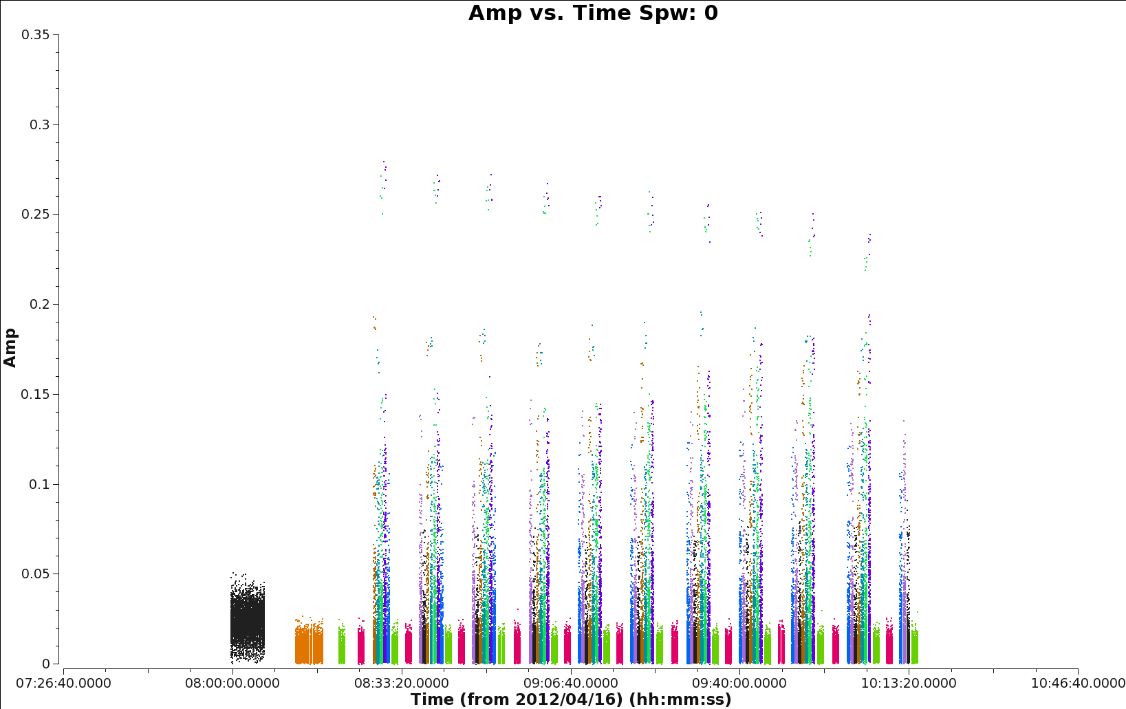
In Figure 5 you can see the output of the following plotms command for data set X39b. By clicking the green arrows in the plotms window you can access all the spws.
# In CASA
# Check overall behavior with time
vis=data[0]
plotms(vis=vis,
       field='',xaxis='time', yaxis='amp',antenna='',
       spw='', avgchannel='3840',coloraxis='field',showgui=True,
       iteraxis='spw',ydatacolumn='data',yselfscale=True)
For the next set of plotms commands, inspect each dataset, noting any problems that you notice.
# In CASA
# For at least one spw go antenna by antenna to look for dropouts not
# obvious in previous plot
vis=data[0]
plotms(vis=vis,
       field='',xaxis='time', yaxis='amp',antenna='',
       spw='2', avgchannel='3840',coloraxis='field',showgui=True,
       iteraxis='antenna',ydatacolumn='data')

# Check out spectral properties of each source for problems
vis=data[0]
plotms(vis=vis,
       field='',xaxis='freq', yaxis='amp',antenna='',
       spw='', avgtime='1e8',avgscan=True,coloraxis='spw',showgui=True,
       iteraxis='field',ydatacolumn='data',yselfscale=False)

# Examine phase of the bandpass calibrator for any problems
vis=data[0]
bp='1924-292'
plotms(vis=vis,
       field=bp,xaxis='freq', yaxis='phase',antenna='',showgui=True,
       spw='', avgtime='1e8',avgscan=True,avgchannel='10',coloraxis='spw',
       iteraxis='baseline',ydatacolumn='data',yselfscale=True)
Flagging
Next, based on our inspection we will proceed with the corresponding flagging. But before that, we will save the current flags state, so we can recover it later, if needed.
# In CASA
data=['uid___A002_X3d4118_X39b.antwvrtsys.ms.fixed',
      'uid___A002_X3d55cb_X575.antwvrtsys.ms.fixed',
      'uid___A002_X3d55cb_X90c.antwvrtsys.ms.fixed',
      'uid___A002_X3d55cb_Xb50.antwvrtsys.ms.fixed']

# Back up flag state in case you want to start over.
for vis in data:
  flagmanager(vis=vis,mode='save',versionname='Original')

# If you need to start over, uncomment and run this section to restore original flags
#for vis in data:
#  flagmanager(vis=vis,mode='restore',versionname='Original')
During the calibration procedure, below, some problems in the data become apparent. When this happens, the problematic data need to be flagged, and then the calibration should be repeated. In order to save you time, however, we will flag those data now.
# In CASA
# PROBLEMS DISCOVERED AFTER INITIAL CALIBRATION INSPECTION

# flag low elevation scans on 1625-254 and IRAS16293
flagdata(vis='uid___A002_X3d55cb_Xb50.antwvrtsys.ms.fixed',
         timerange='>11:54:00', field='',flagbackup=False)

# flag low gains on DV02 on Juno
flagdata(vis='uid___A002_X3d55cb_Xb50.antwvrtsys.ms.fixed',
         antenna='DV02', field='Juno',flagbackup=False)

flagdata(vis='uid___A002_X3d4118_X39b.antwvrtsys.ms.fixed',
         antenna='DV02', field='Juno',flagbackup=False)
Calibration
Now we can start with the calibration itself. First, we will set the flux model and perform the bandpass calibration using 1924-292 and 3c279. As before, we define our list of data and match the sources with intents. You can use the listobs to find the intents listed for each scan and field.
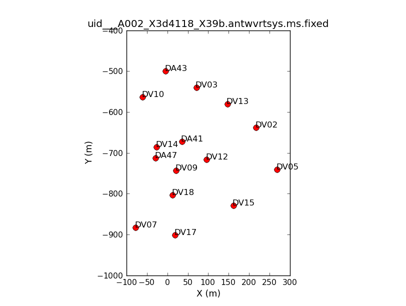
We will set our reference antenna (one close to the center of the array and without problems, like delays). Use plotants to find an antenna close to the center of the array. Figure 6 shows an example plot from execution X39b.
As you can see, two different intervals for channels are used. We use the center channels to calculate the phase variation over the bandpass scan. Later, we want to use all channels except the edge channels to compute the gains and apply them to the science target.
# In CASA
data=['uid___A002_X3d4118_X39b.antwvrtsys.ms.fixed',
      'uid___A002_X3d55cb_X575.antwvrtsys.ms.fixed',
      'uid___A002_X3d55cb_X90c.antwvrtsys.ms.fixed',
      'uid___A002_X3d55cb_Xb50.antwvrtsys.ms.fixed']
# Match up intents with source names
pcal='1625-254'
fluxcal='Juno'
science='IRAS16293*'
check='nrao530*'
bpcal=['1924-292','3c279','1924-292','1924-292']
calfields=['1924-292,Juno,1625-254,nrao530*',
           '3c279,Juno,1625-254,nrao530*',
           '1924-292,Juno,1625-254,nrao530*',
           '1924-292,Juno,1625-254,nrao530*']

# Setup calibration parameters
prebpchan='0~3:1200~1500'
calchan='0~3:20~3820'
refant='DV14'
gaps=5
os.system('rm -rf *cal')
Note that if at some point during the calibration process you need to start over, then you will need to clear all the columns for solutions in the data, as shown next.
The following setjy command sets the model column for the flux calibrator. For CASA 5.3 and later, usescratch should be explicitly set to True for any ephemeris calibrator.
# In CASA
for vis in range(len(data)):
  delmod(vis=data[vis])
  setjy(vis=data[vis],field=fluxcal,standard='Butler-JPL-Horizons 2012',
        scalebychan=True,usescratch=True)
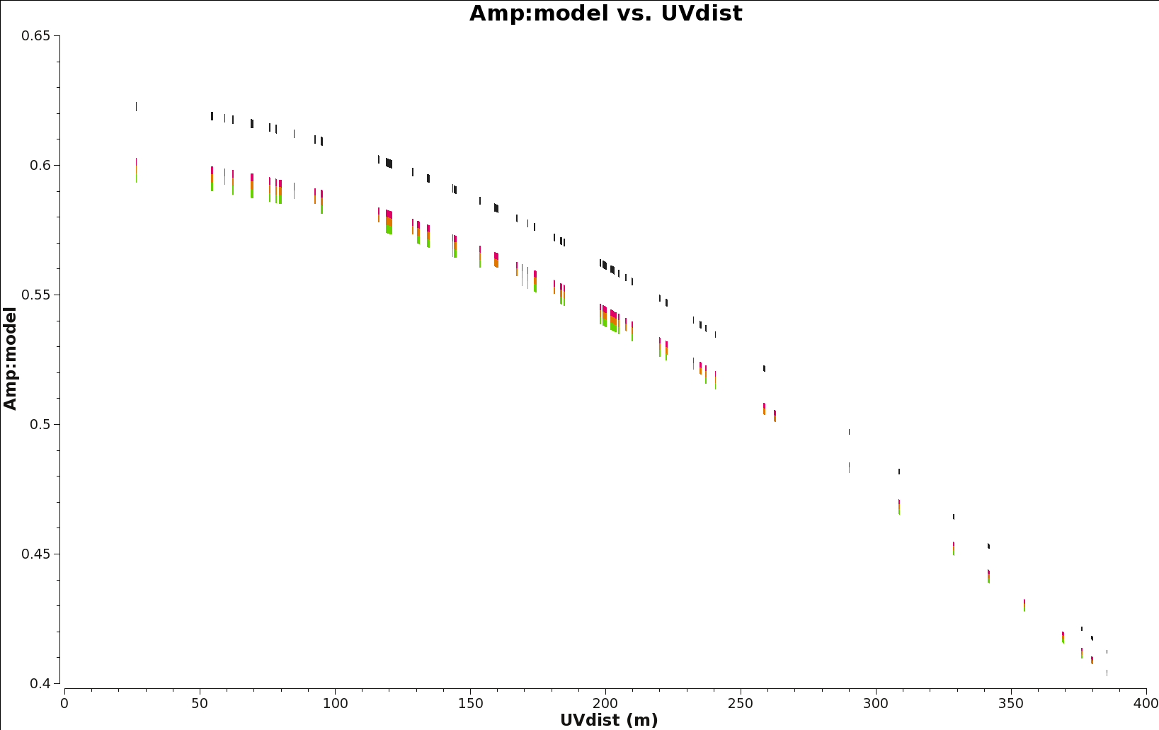
Now we proceed with the bandpass calibration, which will be done in two steps. In the first one, we will use a small block of channels in the center of the spws, 1200~1500, to calculate gains in phase, using a solution interval of 30 seconds. This will give us the variation of the phase throughout the observation. We will use this table later to execute the bandpass itself. Note that we are using a minimum signal to noise ratio of 2 to accept the solutions. This is low but necessary since the calibrators are not very strong in band 9.
# In CASA
# Calculating phase variation with time
for vis in range(len(data)):
  gaincal(vis=data[vis],caltable=data[vis]+'.bpphase.gcal',
        field=bpcal[vis],spw=prebpchan,refant=refant,
        calmode='p',solint='30s',minsnr=2.0,minblperant=4)
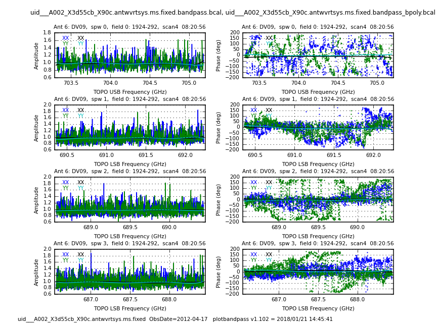
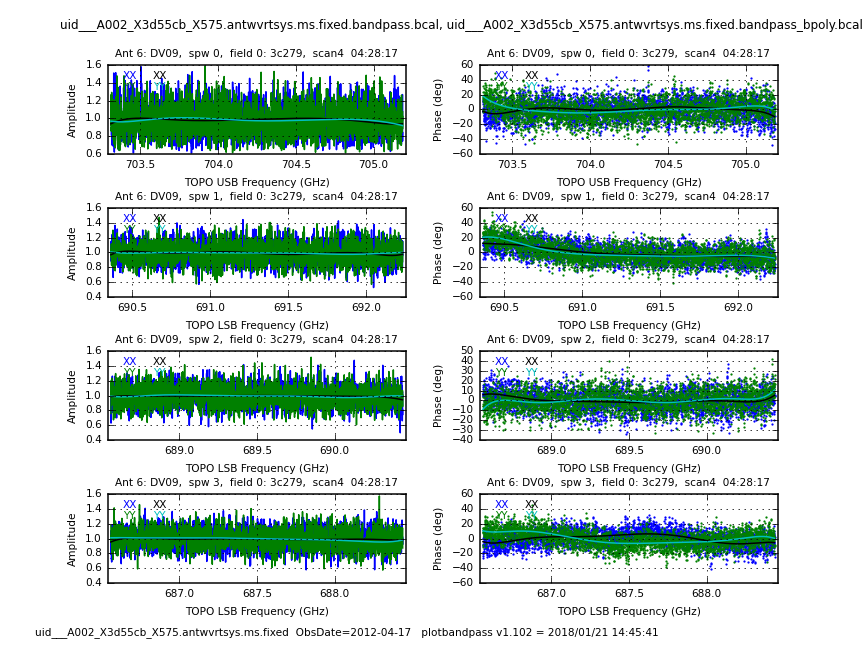
Next, we set our bandpass command to use our previously generated gain tables. Since we do not have a high signal to noise ratio per channel, we use a polynomial option to calculate the solutions for the bandpass. In the bandpass task, the options degamp and degphase will set the maximum degree of the polynomial that the task can use to calculate solutions. In the CASA log you can note what is the actual degree that the task is using. Note that the combination of solint='inf' and combine='scan' will result in one solution per scan for the calibrator. Even with these modifications, you will see some warnings about low SNR. Data with too low SNR will be flagged.
# In CASA
# Bandpass calibration using previous tables as input
for vis in range(len(data)):
  bandpass(vis=data[vis],caltable=data[vis]+'.bandpass.bcal',
        field=bpcal[vis],spw='',combine='scan',refant=refant,
        solint='inf',solnorm=True,minblperant=4,fillgaps=gaps,
        gaintable=[data[vis]+'.bpphase.gcal'])

for vis in range(len(data)):
  bandpass(vis=data[vis],caltable=data[vis]+'.bandpass_bpoly.bcal',
        field=bpcal[vis],spw='',combine='scan',refant=refant,
        solint='inf',solnorm=True,minblperant=4,fillgaps=gaps,
        bandtype='BPOLY',degamp=7,degphase=7,
        gaintable=[data[vis]+'.bpphase.gcal'])
To plot all our tables we will use plotbandpass and plotms. The plotbandpass command will create plot files for each combination of dataset and antenna, for both amplitude and phase. Inspect all these plots to make sure that the bandpass solutions look good. In Figures 8 and 9 we show an output sample for this command for the two bandpass calibrators used -- note how noisy the weaker bandpass calibrator (J1924) is without BPOLY.
# In CASA
# Set some plotting things
SPW=['0','1','2','3']
numants=15 # max for any of the input datasets
os.system('rm -rf cal_plots')
os.system('mkdir cal_plots')

os.system('rm -rf cal_plots/*bandpass_bpoly.bcal.*png')
for vis in range(len(data)):
  plotbandpass(caltable=data[vis]+'.bandpass.bcal',
                caltable2=data[vis]+'.bandpass_bpoly.bcal',
                field=bpcal[vis],xaxis='freq',yaxis='both',
                figfile='cal_plots/'+data[vis]+'.bandpass_bpoly.png',
                interactive=False,subplot=42)
The next step in the calibration is to calculate amplitude and phase gains vs time for our calibrators. The ideal case here is to have a solution per integration of the data, but in this case we will need to use a solution interval of 30 seconds to avoid having many failed solutions, especially in the weak phase calibrator. First, we will calculate gains for phase and later using that information, we will solve for amplitude and phase. In all the next three executions we are using the bandpass calibration table, as it provides the gains for phase and amplitude vs frequency. These solutions will be applied to the calibrators.
# In CASA
#Using 30s (5 integrations) per solution to avoid many failed solution of the weak calibrator.
for vis in range(len(data)):
  gaincal(vis=data[vis],caltable=data[vis]+'.intphase.gcal',
        field=calfields[vis],spw=calchan,refant=refant,
        calmode='p',solint='30s',minsnr=2.0,minblperant=4,
        gaintable=[data[vis]+'.bandpass_bpoly.bcal'])
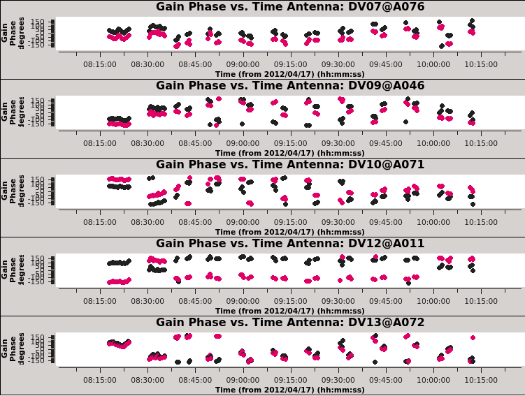
To plot our *.intphase.gcal tables we use the next command, which will create files containing the phase gains vs time for all the antennas and for all the datasets. In Figure 10 we show an example of such plots. Again, you will need to check all plots to make sure the solutions are good. To speed things up, we will loop over the antenna indices and plot 5 antennas per page. Some of the antennas were completely flagged prior to running split; plots for those antennas will be empty.
# In CASA
# Plotting phase gains vs time
os.system('rm -rf cal_plots/*intphase*png')
for vis in data:
  for spw in SPW:
    for antenna in range(0,numants,5):
        plotms(vis=vis+'.intphase.gcal',
             xaxis='time',yaxis='phase',antenna='%d~%d'%(antenna,antenna+4),spw=spw,
             iteraxis='antenna',gridrows=5,gridcols=1,coloraxis='corr',
             showgui=False,
             plotfile='cal_plots/'+vis+'.intphase.gcal.spw%s.ant%d_%d.png'%(spw,antenna,antenna+4),
             plotrange=[0,0,-180,180])
Next we will use gaincal to solve for gain phases for all the calibrators, but this time we will get one single solution per scan. These solutions will be applied to the science target.
# In CASA
# Gaincal execution as before, but to get a single solution per scan
for vis in range(len(data)):
  gaincal(vis=data[vis],caltable=data[vis]+'.scanphase.gcal',
        field=calfields[vis],spw=calchan,refant=refant,
        calmode='p',solint='inf',minsnr=2.0,minblperant=4,
        gaintable=[data[vis]+'.bandpass_bpoly.bcal'])
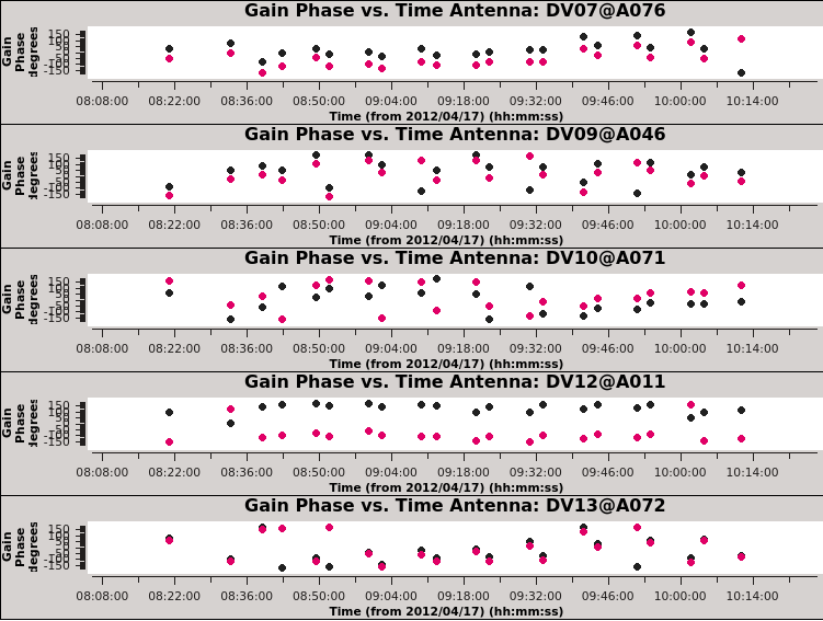
The next command will produce many plots, and like the previous one, you will get one for each dataset and for each antenna. See example in Figure 11.
# In CASA
# Phase vs time plotting for our calibrators
os.system('rm -rf cal_plots/*scanphase*png')
for vis in data:
  for spw in SPW:
    for antenna in range(0,numants,5):
        plotms(vis=vis+'.scanphase.gcal',
            xaxis='time',yaxis='phase',antenna='%d~%d'%(antenna,antenna+4),
            iteraxis='antenna',gridrows=5,gridcols=1,coloraxis='corr',spw=spw,
            showgui=False,
            plotfile='cal_plots/'+vis+'.scanphase.gcal.spw%s.ant%d_%d.png'%(spw,antenna,antenna+4),
            plotrange=[0,0,-180,180])
Finally, in the next gaincal we will solve for amplitude and phase. We will use the gain phase calibration table produced before. We will get one solution per scan for all our calibrators.
# In CASA
# Gaincal solving for amplitude and phase vs time.
for vis in range(len(data)):
  gaincal(vis=data[vis],caltable=data[vis]+'.amp.gcal',
        field=calfields[vis],spw=calchan,refant=refant,
        calmode='ap',solint='inf',minsnr=2.0,minblperant=4,
        gaintable=[data[vis]+'.bandpass_bpoly.bcal',data[vis]+'.intphase.gcal'])
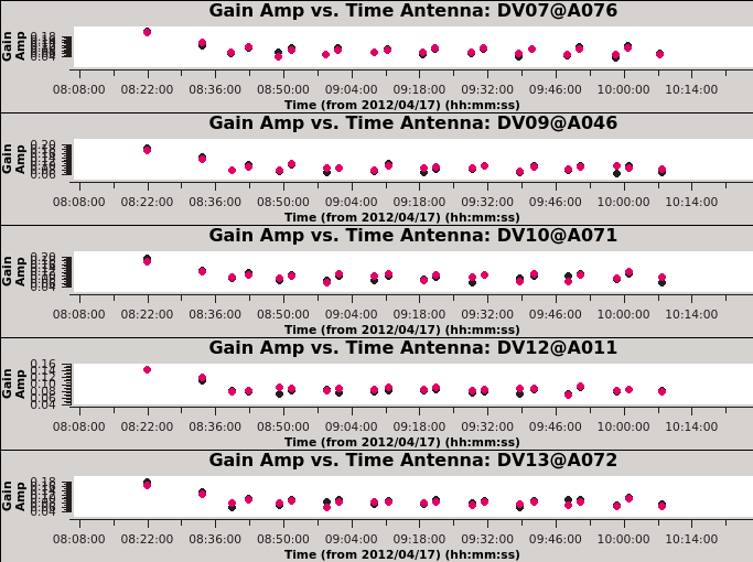
We now can check the resulting plots with the next plotms executions. In Figure 12 we show an example of these plots.
# In CASA
# Plotting gain amplitudes as function of time.
os.system('rm -rf cal_plots/*amp*png')
for vis in data:
  for spw in SPW:
    for antenna in range(0,numants,5):
        plotms(vis=vis+'.amp.gcal',
            xaxis='time',yaxis='amp',antenna='%d~%d'%(antenna,antenna+4),
            iteraxis='antenna',gridrows=5,gridcols=1,spw=spw,coloraxis='corr',
            plotfile='cal_plots/'+vis+'.amp.gcal.spw%s.ant%d_%d.png'%(spw,antenna,antenna+4),
            showgui=True)
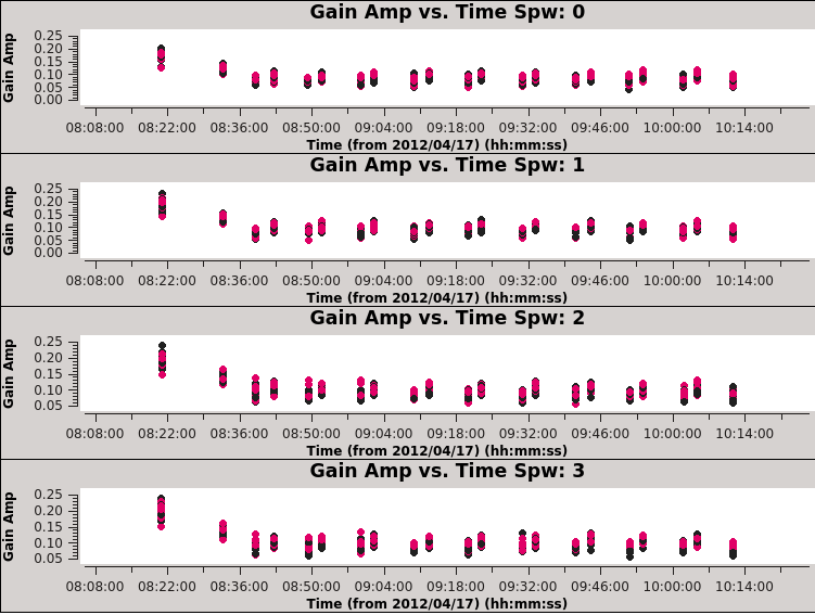
We can plot the same tables but in a different way that will allow us to look for higher abnormal gains in the solutions. With the next command we will get only four plots for each spw. Each of those plots shows all the gains for all the antennas for all the sources (See Figure 13 for an example). Below in the box, there are some comments to focus you on some data, so you can double check. Before continuing, make sure you check all the calibration tables.
# In CASA
# Look for low or high gains compared to other data
os.system('rm -rf *amp.png')
for vis in data:
    plotms(vis=vis+'.amp.gcal',
            xaxis='time',yaxis='amp',antenna='',field='',
            iteraxis='spw',gridrows=4,gridcols=1,spw='',coloraxis='corr',
            showgui=False,plotfile=vis+'.amp.png')

# X90c shows no issues
# X575 shows no issues
# Xb50 shows bad end times for all spws (due to low el). spw=0 is worse than other spw.
# X39b shows no issues
Set Absolute Flux Scale
Now that the gain calibration is done, we need to set the flux for our calibrators. Remember that we set the model for the flux calibrator prior to deriving the bandpass and gain calibration tables. For this we will use Juno, our primary flux calibrator. We will do this by using fluxscale. We then will transfer the flux information from our phase calibrator to our science target. For these datasets, we note the following for this step: The derived flux densities for X39b, X90c, and Xb50 are quite reasonable. The results for X575 are a little high, probably because Juno was at low elevation for these observations.
# In CASA
# Setting fluxes

for vis in range(len(data)):
  fluxscale(vis=data[vis],caltable=data[vis]+'.amp.gcal',
            fluxtable=data[vis]+'.flux.cal',reference=fluxcal)
Below we copy the fluxscale numbers from the logger window:
##########################################
##### Begin Task: fluxscale          #####
fluxscale( vis='uid___A002_X3d55cb_X575.antwvrtsys.ms.fixed', caltable='uid___A002_X3d55cb_X575.antwvrtsys.ms.fixed.amp.gcal', fluxtable='uid___A002_X3d55cb_X575.antwvrtsys.ms.fixed.flux.cal', reference=['Juno'], transfer=[], listfile='', append=False, refspwmap=[-1], gainthreshold=-1.0, antenna='', timerange='', scan='', incremental=False, fitorder=1, display=False )
****Using NEW VI2-driven calibrater tool****
Opening MS: uid___A002_X3d55cb_X575.antwvrtsys.ms.fixed for calibration.
Initializing nominal selection to the whole MS.
Beginning fluxscale--(MSSelection version)-------
Assuming all non-reference fields are transfer fields.
Found reference field(s): Juno
Found transfer field(s):  3c279 nrao530 ph 1625-254
Flux density for 3c279 in SpW=0 (freq=7.0425e+11 Hz) is: 8.39476 +/- 0.204702 (SNR = 41.0096, N = 22)
Flux density for 3c279 in SpW=1 (freq=6.913e+11 Hz) is: 9.27946 +/- 0.17194 (SNR = 53.9691, N = 22)
Flux density for 3c279 in SpW=2 (freq=6.895e+11 Hz) is: 9.3027 +/- 0.199695 (SNR = 46.5844, N = 20)
Flux density for 3c279 in SpW=3 (freq=6.875e+11 Hz) is: 8.24841 +/- 0.2145 (SNR = 38.4541, N = 20)
Flux density for nrao530 ph in SpW=0 (freq=7.0425e+11 Hz) is: 0.789052 +/- 0.0669805 (SNR = 11.7803, N = 22)
Flux density for nrao530 ph in SpW=1 (freq=6.913e+11 Hz) is: 0.868468 +/- 0.0561378 (SNR = 15.4703, N = 22)
Flux density for nrao530 ph in SpW=2 (freq=6.895e+11 Hz) is: 0.796413 +/- 0.0859909 (SNR = 9.2616, N = 20)
Flux density for nrao530 ph in SpW=3 (freq=6.875e+11 Hz) is: 0.792096 +/- 0.0661582 (SNR = 11.9728, N = 20)
Flux density for 1625-254 in SpW=0 (freq=7.0425e+11 Hz) is: 0.533526 +/- 0.0643791 (SNR = 8.28726, N = 22)
Flux density for 1625-254 in SpW=1 (freq=6.913e+11 Hz) is: 0.56966 +/- 0.0504597 (SNR = 11.2894, N = 22)
Flux density for 1625-254 in SpW=2 (freq=6.895e+11 Hz) is: 0.53882 +/- 0.0579978 (SNR = 9.29035, N = 20)
Flux density for 1625-254 in SpW=3 (freq=6.875e+11 Hz) is: 0.529533 +/- 0.0564098 (SNR = 9.38725, N = 20)
Fitted spectrum for 3c279 with fitorder=1: Flux density = 8.89665 +/- 0.310614 (freq=693.107 GHz) spidx: a_1 (spectral index) =-2.44007 +/- 4.07765 covariance matrix for the fit:  covar(0,0)=0.000121724 covar(0,1)=0.00190679 covar(1,0)=0.00190679 covar(1,1)=8.80316
Fitted spectrum for nrao530 ph with fitorder=1: Flux density = 0.821224 +/- 0.0252078 (freq=693.107 GHz) spidx: a_1 (spectral index) =-1.38781 +/- 3.4266 covariance matrix for the fit:  covar(0,0)=0.00164685 covar(0,1)=0.00179584 covar(1,0)=0.00179584 covar(1,1)=108.809
Fitted spectrum for 1625-254 with fitorder=1: Flux density = 0.545704 +/- 0.0121054 (freq=693.107 GHz) spidx: a_1 (spectral index) =-0.44401 +/- 2.62301 covariance matrix for the fit:  covar(0,0)=0.00274406 covar(0,1)=0.0961512 covar(1,0)=0.0961512 covar(1,1)=203.416
Storing result in uid___A002_X3d55cb_X575.antwvrtsys.ms.fixed.flux.cal
Writing solutions to table: uid___A002_X3d55cb_X575.antwvrtsys.ms.fixed.flux.cal
End task fluxscale
##########################################

##########################################
##### Begin Task: fluxscale          #####
fluxscale( vis='uid___A002_X3d55cb_X90c.antwvrtsys.ms.fixed', caltable='uid___A002_X3d55cb_X90c.antwvrtsys.ms.fixed.amp.gcal', fluxtable='uid___A002_X3d55cb_X90c.antwvrtsys.ms.fixed.flux.cal', reference=['Juno'], transfer=[], listfile='', append=False, refspwmap=[-1], gainthreshold=-1.0, antenna='', timerange='', scan='', incremental=False, fitorder=1, display=False )
Found reference field(s): Juno
Found transfer field(s):  1924-292 nrao530 ph 1625-254
Flux density for 1924-292 in SpW=0 (freq=7.0425e+11 Hz) is: 1.89287 +/- 0.076882 (SNR = 24.6205, N = 22)
Flux density for 1924-292 in SpW=1 (freq=6.913e+11 Hz) is: 1.9873 +/- 0.0658816 (SNR = 30.1647, N = 22)
Flux density for 1924-292 in SpW=2 (freq=6.895e+11 Hz) is: 2.10813 +/- 0.0608377 (SNR = 34.6518, N = 22)
Flux density for 1924-292 in SpW=3 (freq=6.875e+11 Hz) is: 2.11659 +/- 0.0599213 (SNR = 35.3229, N = 22)
Flux density for nrao530 ph in SpW=0 (freq=7.0425e+11 Hz) is: 0.559174 +/- 0.037827 (SNR = 14.7824, N = 22)
Flux density for nrao530 ph in SpW=1 (freq=6.913e+11 Hz) is: 0.57902 +/- 0.0342671 (SNR = 16.8973, N = 22)
Flux density for nrao530 ph in SpW=2 (freq=6.895e+11 Hz) is: 0.62241 +/- 0.030583 (SNR = 20.3515, N = 22)
Flux density for nrao530 ph in SpW=3 (freq=6.875e+11 Hz) is: 0.608023 +/- 0.0334248 (SNR = 18.1908, N = 22)
Flux density for 1625-254 in SpW=0 (freq=7.0425e+11 Hz) is: 0.380802 +/- 0.0324843 (SNR = 11.7226, N = 22)
Flux density for 1625-254 in SpW=1 (freq=6.913e+11 Hz) is: 0.385912 +/- 0.0264433 (SNR = 14.594, N = 22)
Flux density for 1625-254 in SpW=2 (freq=6.895e+11 Hz) is: 0.397979 +/- 0.029181 (SNR = 13.6383, N = 22)
Flux density for 1625-254 in SpW=3 (freq=6.875e+11 Hz) is: 0.381872 +/- 0.0272565 (SNR = 14.0103, N = 22)
Fitted spectrum for 1924-292 with fitorder=1: Flux density = 2.02625 +/- 0.0264888 (freq=693.107 GHz) spidx: a_1 (spectral index) =-4.72937 +/- 1.56847 covariance matrix for the fit:  covar(0,0)=0.000272966 covar(0,1)=0.0207808 covar(1,0)=0.0207808 covar(1,1)=20.833
Fitted spectrum for nrao530 ph with fitorder=1: Flux density = 0.593166 +/- 0.00993785 (freq=693.107 GHz) spidx: a_1 (spectral index) =-3.95157 +/- 1.96677 covariance matrix for the fit:  covar(0,0)=0.000833282 covar(0,1)=0.0446335 covar(1,0)=0.0446335 covar(1,1)=60.8832
Fitted spectrum for 1625-254 with fitorder=1: Flux density = 0.386509 +/- 0.00442442 (freq=693.107 GHz) spidx: a_1 (spectral index) =-0.751283 +/- 1.3282 covariance matrix for the fit:  covar(0,0)=0.001395 covar(0,1)=0.0548219 covar(1,0)=0.0548219 covar(1,1)=99.5728
Storing result in uid___A002_X3d55cb_X90c.antwvrtsys.ms.fixed.flux.cal
Writing solutions to table: uid___A002_X3d55cb_X90c.antwvrtsys.ms.fixed.flux.cal
##### End Task: fluxscale            #####
##########################################

##########################################
##### Begin Task: fluxscale          #####
fluxscale( vis='uid___A002_X3d55cb_Xb50.antwvrtsys.ms.fixed', caltable='uid___A002_X3d55cb_Xb50.antwvrtsys.ms.fixed.amp.gcal', fluxtable='uid___A002_X3d55cb_Xb50.antwvrtsys.ms.fixed.flux.cal', reference=['Juno'], transfer=[], listfile='', append=False, refspwmap=[-1], gainthreshold=-1.0, antenna='', timerange='', scan='', incremental=False, fitorder=1, display=False )
Found reference field(s): Juno
Found transfer field(s):  1924-292 nrao530 ph 1625-254
Flux density for 1924-292 in SpW=0 (freq=7.0425e+11 Hz) is: 2.25348 +/- 0.0605347 (SNR = 37.2263, N = 22)
Flux density for 1924-292 in SpW=1 (freq=6.913e+11 Hz) is: 2.26898 +/- 0.0446163 (SNR = 50.8553, N = 22)
Flux density for 1924-292 in SpW=2 (freq=6.895e+11 Hz) is: 2.08406 +/- 0.0504538 (SNR = 41.3064, N = 22)
Flux density for 1924-292 in SpW=3 (freq=6.875e+11 Hz) is: 2.15783 +/- 0.0523674 (SNR = 41.2056, N = 22)
Flux density for nrao530 ph in SpW=0 (freq=7.0425e+11 Hz) is: 0.666662 +/- 0.048484 (SNR = 13.7501, N = 22)
Flux density for nrao530 ph in SpW=1 (freq=6.913e+11 Hz) is: 0.615613 +/- 0.0383819 (SNR = 16.0391, N = 22)
Flux density for nrao530 ph in SpW=2 (freq=6.895e+11 Hz) is: 0.623548 +/- 0.0407315 (SNR = 15.3087, N = 22)
Flux density for nrao530 ph in SpW=3 (freq=6.875e+11 Hz) is: 0.639782 +/- 0.0390136 (SNR = 16.399, N = 22)
Flux density for 1625-254 in SpW=0 (freq=7.0425e+11 Hz) is: 0.439408 +/- 0.0492581 (SNR = 8.92051, N = 22)
Flux density for 1625-254 in SpW=1 (freq=6.913e+11 Hz) is: 0.433931 +/- 0.0303049 (SNR = 14.3188, N = 22)
Flux density for 1625-254 in SpW=2 (freq=6.895e+11 Hz) is: 0.417476 +/- 0.0390596 (SNR = 10.6882, N = 22)
Flux density for 1625-254 in SpW=3 (freq=6.875e+11 Hz) is: 0.421725 +/- 0.0320614 (SNR = 13.1537, N = 22)
Fitted spectrum for 1924-292 with fitorder=1: Flux density = 2.20084 +/- 0.0473314 (freq=693.107 GHz) spidx: a_1 (spectral index) =2.03197 +/- 2.54039 covariance matrix for the fit:  covar(0,0)=0.000137471 covar(0,1)=0.00439531 covar(1,0)=0.00439531 covar(1,1)=10.17
Fitted spectrum for nrao530 ph with fitorder=1: Flux density = 0.635998 +/- 0.0090556 (freq=693.107 GHz) spidx: a_1 (spectral index) =2.36693 +/- 1.61323 covariance matrix for the fit:  covar(0,0)=0.00107029 covar(0,1)=0.0354117 covar(1,0)=0.0354117 covar(1,1)=72.8453
Fitted spectrum for 1625-254 with fitorder=1: Flux density = 0.429361 +/- 0.00401286 (freq=693.107 GHz) spidx: a_1 (spectral index) =1.81501 +/- 1.17525 covariance matrix for the fit:  covar(0,0)=0.0018959 covar(0,1)=0.152973 covar(1,0)=0.152973 covar(1,1)=158.945
Storing result in uid___A002_X3d55cb_Xb50.antwvrtsys.ms.fixed.flux.cal
Writing solutions to table: uid___A002_X3d55cb_Xb50.antwvrtsys.ms.fixed.flux.cal
##### End Task: fluxscale            #####
When derived fluxes are too high and nothing else appears wrong with the data, the cause (especially at Band 9) is likely to be decorrelation. So we will use the lower values to explicitly set the flux densities based on the fluxscale results. We set the flux of the two bandpass calibrators for the convenience of having a fully calibrated dataset. The only ones that really matter are 1625 as the gain calibrator and the check source nrao530. Based on this, we proceed as follows to make the changes that are needed:
# In CASA
# Fixing the fluxes
flux1924=[2.11,0,0,0]
flux1625=[0.43,0,0,0]
fluxnrao530=[0.66,0,0,0]
flux3c279=[8.89,0,0,0]

datawith1924=['uid___A002_X3d4118_X39b.antwvrtsys.ms.fixed',
      'uid___A002_X3d55cb_X90c.antwvrtsys.ms.fixed',
      'uid___A002_X3d55cb_Xb50.antwvrtsys.ms.fixed']
for vis in datawith1924:
  setjy(vis=vis,field='1924-292',standard='manual',fluxdensity=flux1924,usescratch=False)
  setjy(vis=vis,field='1625-254',standard='manual',fluxdensity=flux1625,usescratch=False)
  setjy(vis=vis,field='nrao530*',standard='manual',fluxdensity=fluxnrao530,usescratch=False)

datawith3c279=['uid___A002_X3d55cb_X575.antwvrtsys.ms.fixed']
for vis in datawith3c279:
  setjy(vis=vis,field='3c279',standard='manual',fluxdensity=flux3c279,usescratch=False)
  setjy(vis=vis,field='1625-254',standard='manual',fluxdensity=flux1625,usescratch=False)
  setjy(vis=vis,field='nrao530*',standard='manual',fluxdensity=fluxnrao530,usescratch=False)
We now need to re-run the amplitude calibration step.
# In CASA
#This new amplitude calibration will be used in the applycal.

data=['uid___A002_X3d4118_X39b.antwvrtsys.ms.fixed',
      'uid___A002_X3d55cb_X575.antwvrtsys.ms.fixed',
      'uid___A002_X3d55cb_X90c.antwvrtsys.ms.fixed',
      'uid___A002_X3d55cb_Xb50.antwvrtsys.ms.fixed']
# Match up intents with source names
pcal='1625-254'
fluxcal='Juno'
science='IRAS16293*'
check='nrao530*'
bpcal=['1924-292','3c279','1924-292','1924-292']
calfields=['1924-292,Juno,1625-254,nrao530*',
           '3c279,Juno,1625-254,nrao530*',
           '1924-292,Juno,1625-254,nrao530*',
           '1924-292,Juno,1625-254,nrao530*']

calchan='0~3:20~3820'
refant='DV14'

for vis in range(len(data)):
  gaincal(vis=data[vis],caltable=data[vis]+'.amp.final.gcal',
        field=calfields[vis],spw=calchan,refant=refant,
        calmode='ap',solint='inf',minsnr=2.0,minblperant=4,
        gaintable=[data[vis]+'.bandpass_bpoly.bcal',data[vis]+'.intphase.gcal'])
Application of calibration tables
Now that we have all the calibration tables with the results, both for gains and flux, we need to apply all the tables to the data. First, we save the state of the flags.
# In CASA
data=['uid___A002_X3d4118_X39b.antwvrtsys.ms.fixed',
      'uid___A002_X3d55cb_X575.antwvrtsys.ms.fixed',
      'uid___A002_X3d55cb_X90c.antwvrtsys.ms.fixed',
      'uid___A002_X3d55cb_Xb50.antwvrtsys.ms.fixed']
# Match up intents with source names
pcal='1625-254'
fluxcal='Juno'
science='IRAS16293*'
check='nrao530*'
bpcal=['1924-292','3c279','1924-292','1924-292']

for vis in range(len(data)):
  flagmanager(vis=data[vis],mode='save',versionname='beforeapplycal')

for vis in range(len(data)):
  applycal(vis=data[vis],field=bpcal[vis],
        gaintable=[data[vis]+'.bandpass_bpoly.bcal',data[vis]+'.intphase.gcal',
                   data[vis]+'.amp.final.gcal'],
        interp=['nearest','nearest','nearest'],
        gainfield=[bpcal[vis],bpcal[vis],bpcal[vis]],flagbackup=False,calwt=False)

for vis in range(len(data)):
  applycal(vis=data[vis],field=pcal,
         gaintable=[data[vis]+'.bandpass_bpoly.bcal',data[vis]+'.intphase.gcal',
                    data[vis]+'.amp.final.gcal'],
        interp=['nearest','nearest','nearest'],
         gainfield=[bpcal[vis],pcal,pcal],flagbackup=False,calwt=False)

for vis in range(len(data)):
  applycal(vis=data[vis],field=fluxcal,
         gaintable=[data[vis]+'.bandpass_bpoly.bcal',data[vis]+'.intphase.gcal',
                    data[vis]+'.amp.final.gcal'],
        interp=['nearest','nearest','nearest'],
         gainfield=[bpcal[vis],fluxcal,fluxcal],flagbackup=False,calwt=False)

for vis in range(len(data)):
  applycal(vis=data[vis],field=science,
        interp=['nearest','linear','linear'],
        gaintable=[data[vis]+'.bandpass_bpoly.bcal',data[vis]+'.scanphase.gcal',
                   data[vis]+'.amp.final.gcal'],
        gainfield=[bpcal[vis],pcal,pcal],flagbackup=False,calwt=False)

for vis in range(len(data)):
  applycal(vis=data[vis],field=check,
        interp=['nearest','linear','linear'],
        gaintable=[data[vis]+'.bandpass_bpoly.bcal',data[vis]+'.scanphase.gcal',
                   data[vis]+'.amp.final.gcal'],
        gainfield=[bpcal[vis],pcal,pcal],flagbackup=False,calwt=False)
Plot corrected data
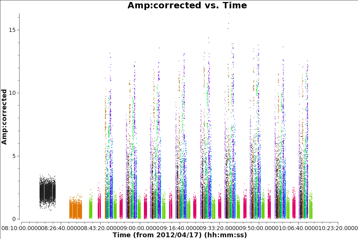
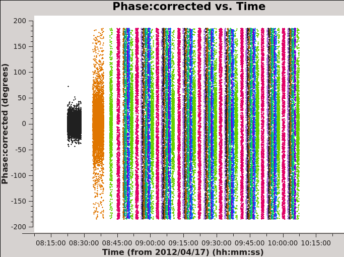
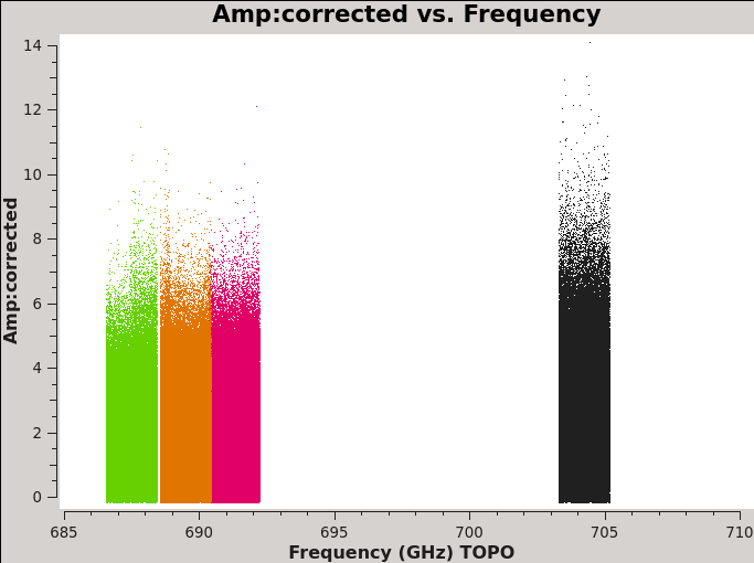
The next commands will help you visualize the result of the application of the calibration tables to the data. You can check if the amplitudes and phases vs time and frequency look reasonable for all the sources, in particular for the science target fields.
The next command will produce four plots, as the one we showed in Figure 5, but the amplitude in these new plots corresponds to flux because we now have calibrated data. See Figure 14 for an example of it. It is important to check that all the sources have similar amplitude (flux) in the different spws and datasets.
# In CASA
data=['uid___A002_X3d4118_X39b.antwvrtsys.ms.fixed',
      'uid___A002_X3d55cb_X575.antwvrtsys.ms.fixed',
      'uid___A002_X3d55cb_X90c.antwvrtsys.ms.fixed',
      'uid___A002_X3d55cb_Xb50.antwvrtsys.ms.fixed']
# Match up intents with source names
pcal='1625-254'
fluxcal='Juno'
science='IRAS16293*'
check='nrao530*'
bpcal=['1924-292','3c279','1924-292','1924-292']
calfields=['1924-292,Juno,1625-254,nrao530*',
           '3c279,Juno,1625-254,nrao530*',
           '1924-292,Juno,1625-254,nrao530*',
           '1924-292,Juno,1625-254,nrao530*']
# Set some plotting things
SPW=['0','1','2','3']

os.system('rm -rf aftercal_plots')
os.system('mkdir aftercal_plots')

os.system('rm -rf aftercal_plots/*cal.time*.png')
for vis in range(len(data)):
  for spw in SPW:
    plotms(vis=data[vis],spw=spw,xaxis='time',yaxis='amp',field='',avgchannel='3840',
       coloraxis='field',ydatacolumn='corrected',showgui=True,
       plotfile='aftercal_plots/'+data[vis]+'.cal.time.spw%s.png'%(spw))
    user_check=input('Press enter to continue script\n')
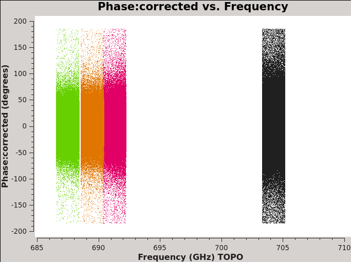
It is also important to check the phases vs time for all the sources. The next command will get you the corresponding plots, four for each dataset. You can see that while the bandpass and amplitude calibrator have very concentrated phases around 0 degrees, the phase calibrator and the science target do not. This is because the bandpass and amplitude calibrators have a higher signal-to-noise than the phase calibrator and science target. In Figure 15 we show an example of these plots for spw 1 in the dataset X90c.
# In CASA
os.system('rm -rf aftercal_plots/*cal.time.phase*.png')
for vis in range(len(data)):
  for spw in SPW:
    plotms(vis=data[vis],spw=spw,xaxis='time',yaxis='phase',field='',avgchannel='3840',
       coloraxis='field',ydatacolumn='corrected',showgui=True,
       plotfile='aftercal_plots/'+data[vis]+'.cal.time.phase.spw%s.png'%(spw))
We now check the amplitude of the sources vs frequency. This is important since we expect that all the spw have very similar behavior. You will have one plot for each field for each dataset. In Figure 16 we show the case for 1625-254, our phase calibrator, for X39b.
# In CASA
os.system('rm -rf aftercal_plots/*cal.freq.amp*.png')
for vis in range(len(data)):
  for field in calfields[vis].split(','):
    plotms(vis=data[vis],field='%s'%field,xaxis='freq', yaxis='amp',
       spw='',avgtime='1e8',avgscan=True,showgui=True,
       coloraxis='spw',xselfscale=True,ydatacolumn='corrected',
       plotfile='aftercal_plots/'+data[vis]+'.cal.freq.amp.'+field+'.png')
The next command will produce similar plots but this time of phase vs frequency (see Figure 17 for an example). You will notice that only strong sources, like 3c279, will show clearly phases concentrated around 0 degrees.
# In CASA
os.system('rm -rf aftercal_plots/*cal.freq.phase*.png')
for vis in range(len(data)):
  for field in calfields[vis].split(','):
    plotms(vis=data[vis],field='%s'%field,xaxis='freq', yaxis='phase',
       spw='',avgtime='1e8',avgscan=True,showgui=True,
       coloraxis='spw',xselfscale=True,ydatacolumn='corrected',
       plotfile='aftercal_plots/'+data[vis]+'.cal.freq.phase.'+field+'.png')
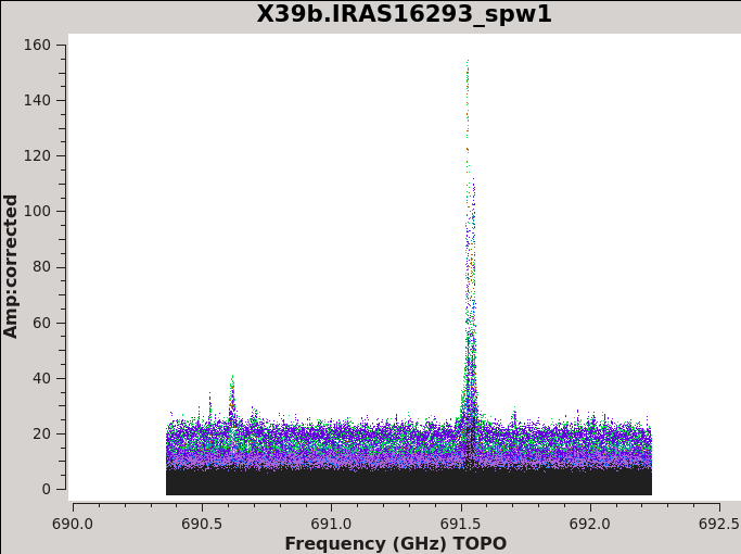
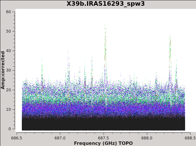
Finally, for our science target, we plot amplitude (flux) vs frequency for all the spectral windows. See an example of this is Figure 18 and 19. If you look carefully at these plots, you will notice that the datasets at low elevation show much more line emission - this is due to the shorter projected baselines present for these datasets (X39b and Xb50). In contrast, you start to see some weak absorption for the dataset at high elevation: X90c.
# In CASA
os.system('rm -rf aftercal_plots/*science.freq.amp*.png')
for vis in range(len(data)):
  for spw in SPW:
    plotms(vis=data[vis],field=science,xaxis='freq', yaxis='amp',
       spw=spw,avgtime='1e8',avgscan=True,showgui=True,
       coloraxis='field',xselfscale=True,ydatacolumn='corrected',
       plotfile='aftercal_plots/'+data[vis]+'.science.freq.amp'+spw+'.png',
       title=data[vis].split('_')[-1].split('.')[0]+'.IRAS16293_spw'+spw)
Next, we put a list of a subset of the same plotms commands that do not produce .png files, but that you can explore using locate and other features available in the GUI.
# In CASA
# Additional manual plots
vis=data[0]
plotms(vis=vis,spw='',xaxis='time',yaxis='amp',field='',avgchannel='3840',
       coloraxis='field',ydatacolumn='corrected',iteraxis='spw',showgui=True)

vis=data[1]
plotms(vis=vis,field=bpcal[1],xaxis='freq', yaxis='amp',
       spw='2',avgtime='1e8',avgscan=True,iteraxis='antenna',
       coloraxis='field',xselfscale=True,ydatacolumn='corrected',showgui=True)

vis=data[1]
plotms(vis=vis,field=calfields[1],xaxis='freq', yaxis='amp',
       spw='',avgtime='1e8',avgscan=True,showgui=True,
       coloraxis='field',xselfscale=True,ydatacolumn='corrected')
Split and concatenate the calibrated data
You are ready now to extract the final calibrated data for the science target. Of course, you can do something similar for the calibrators if you are interested.
# In CASA
# Splitting final calibrated datasets
data=['uid___A002_X3d4118_X39b.antwvrtsys.ms.fixed',
      'uid___A002_X3d55cb_X575.antwvrtsys.ms.fixed',
      'uid___A002_X3d55cb_X90c.antwvrtsys.ms.fixed',
      'uid___A002_X3d55cb_Xb50.antwvrtsys.ms.fixed']

for vis in data:
  split(vis=vis,outputvis='%s.cal.IRAS16293.ms.fixed'%(vis.split('.')[0]),
     datacolumn='corrected',field='IRAS16293*',keepflags=False)
There are now four datasets fully calibrated. We finally will merge these datasets into a single one, in order to proceed with the analysis and imaging in both continuum and spectral line.
# In CASA
# Concatenating the final split files
concatdata=['uid___A002_X3d4118_X39b.cal.IRAS16293.ms.fixed',
     'uid___A002_X3d55cb_X575.cal.IRAS16293.ms.fixed',
     'uid___A002_X3d55cb_X90c.cal.IRAS16293.ms.fixed',
     'uid___A002_X3d55cb_Xb50.cal.IRAS16293.ms.fixed']

concat(vis=concatdata,concatvis='IRAS16293_Band9.fixed.ms')
To speed up imaging we apply 60 second time averaging to the concatenated dataset.
# In CASA
# 60s time averaging
split(vis='IRAS16293_Band9.fixed.ms', datacolumn='data', timebin='60s',
       outputvis='IRAS16293_Band9.fixed.rebin.ms')
As a final step, we zero the rows of the pointing table because it is quite large and is not currently needed by the imaging software for mosaics -indeed its presence will cause an error during imaging if you skip this step.
# In CASA
# Remove rows of pointing table
tb.open('IRAS16293_Band9.fixed.rebin.ms/POINTING', nomodify = False)
a = tb.rownumbers()
tb.removerows(a)
tb.close()
Now you have completed the calibration and have everything you need to carry out the imaging stage. Follow IRAS16293 Band9 - Imaging to go to the imaging section of this casaguide.
Last checked on CASA Version 6.4.1