M100 Band3 SingleDish 4.3
- This guide requires CASA 4.3 and assumes that you have downloaded M100_Band3_TP_UncalibratedData.tgz as described in M100_Band3#Obtaining_the_Data
- Details of the ALMA observations are described at M100_Band3
- This portion of the guide covers calibration and imaging starting from the raw visibility data.
Overview
This portion of CASA Guide will cover the data reduction of the Total Power (TP) array observations of M100. The data consist of "amplitude calibrator" datasets (containing observational data of the quasar 3C279) and "science" datasets containing data for the science target M100. The data are reduced in the following steps:
- Both the amplitude calibrator and science datasets are calibrated into units of Kelvins.
- The radio continuum emission from 3C279 in the amplitude calibrator data are used to derive the Jansky/Kelvin (Jy/K) factors for individual days and frequencies (spectral windows).
- Using the derived Jy/K values, the science data are calibrated into Jy/beam units.
- The calibrated science data are imaged into a data cube.
The combination of the resultant image with the interferometric (12-m array and 7-m array) data is explained in a separate page M100_Band3_Combine_4.3.
This guide is designed for CASA 4.3.0.
Confirm Your Version of CASA
This guide has been written for CASA release 4.3.0. Please confirm your version before proceeding.
# In CASA
version = casadef.casa_version
print "You are using " + version
if (version < '4.3.0'):
    print "YOUR VERSION OF CASA IS TOO OLD FOR THIS GUIDE."
    print "PLEASE UPDATE IT BEFORE PROCEEDING."
else:
    print "Your version of CASA is appropriate for this guide."
Import "Analysis Utilities"
The Analysis_Utilities package will be used for the following processes. Import the package and instantiate the stuffForScienceDataReduction class therein.
# In CASA
import analysisUtils as aU
es = aU.stuffForScienceDataReduction()
Summary of Datasets
The observations were made on the 1st, 5th, 7th, and 17th July 2014, using two or three 12-m antennas and the ACA correlator. The table below indicates the ID's of the Execution Blocks, their start and end times, and the antennas in the array. There are nine science datasets (i.e., two or three per day).
#Science
uid___A002_X85c183_X36f      Observed from 2014-07-01T21:51:26.2 to 2014-07-01T22:40:28.4 (UTC)      DA61, PM03, PM04
uid___A002_X85c183_X60b      Observed from 2014-07-01T22:43:50.0 to 2014-07-01T23:32:39.6 (UTC)      DA61, PM03, PM04
uid___A002_X8602fa_X2ab      Observed from 2014-07-05T23:58:03.6 to 2014-07-06T00:46:52.0 (UTC)      PM02, PM03, PM04
uid___A002_X8602fa_X577      Observed from 2014-07-06T00:55:17.8 to 2014-07-06T01:44:07.3 (UTC)      PM02, PM03, PM04
uid___A002_X864236_X2d4      Observed from 2014-07-07T23:03:48.1 to 2014-07-07T23:53:47.9 (UTC)      PM03, PM04
uid___A002_X864236_X693      Observed from 2014-07-07T23:56:09.6 to 2014-07-08T00:46:07.1 (UTC)      PM03, PM04
uid___A002_X86fcfa_Xd9       Observed from 2014-07-17T20:55:15.5 to 2014-07-17T21:44:06.1 (UTC)      DV10, PM03, PM04
uid___A002_X86fcfa_X664      Observed from 2014-07-17T22:24:17.3 to 2014-07-17T23:13:08.0 (UTC)      DV10, PM03, PM04
uid___A002_X86fcfa_X96c      Observed from 2014-07-17T23:23:37.0 to 2014-07-18T00:12:25.3 (UTC)      DV10, PM03, PM04
Here we define the list of the Execution Block ID's of the science datasets, to facilitate data reduction using for-loops.
# In CASA
basename_science = ['uid___A002_X85c183_X36f', 'uid___A002_X85c183_X60b',
                    'uid___A002_X8602fa_X2ab', 'uid___A002_X8602fa_X577',
                    'uid___A002_X864236_X2d4', 'uid___A002_X864236_X693',
                    'uid___A002_X86fcfa_Xd9', 'uid___A002_X86fcfa_X664',
                    'uid___A002_X86fcfa_X96c']
Calibration into Brightness Temperature in Kelvins
In this section, the data are calibrated into brightness temperature in units of K.
This is done in the steps that are described below, using uid___A002_X85c183_X36f as an example. If you wish to simply calibrate the data without working through the steps, you can instead execute the script A002_X85c183_X36f.ms.scriptForSDCalibration.py using the execfile command.
# In CASA
execfile('A002_X85c183_X36f.ms.scriptForSDCalibration.py')
The other datasets also need to be calibrated using the following scripts; A002_X85c183_X60b.ms.scriptForSDCalibration.py, A002_X8602fa_X2ab.ms.scriptForSDCalibration.py, A002_X8602fa_X577.ms.scriptForSDCalibration.py, A002_X8602fa_X2d4.ms.scriptForSDCalibration.py, A002_X864236_X693.ms.scriptForSDCalibration.py, A002_X86fcfa_Xd9.ms.scriptForSDCalibration.py, A002_X86fcfa_X664.ms.scriptForSDCalibration.py, and A002_X86fcfa_X96c.ms.scriptForSDCalibration.py. The following piece of code executes these scripts.
# In CASA
for basename in basename_science:
    scriptname = basename[6:]+'.ms.scriptForSDCalibration.py'
    if basename == 'uid___A002_X85c183_X36f':
        print 'Calibration procedure for %s is described in the Guide.' % basename
        print 'Please go through the Guide, '
        print 'or run  execfile("%s")  instead.' % scriptname
    else:
        print 'Calibrating %s ...' % basename
        execfile(scriptname)
Import the Data
The first thing to do is to convert the dataset into the CASA Measurement Set (MS) format. The raw data have been provided to you in the ASDM (ALMA Science Data Model). It is the native format of the data produced by the observatory but cannot be processed by CASA. The conversion from ASDM to MS is done with the task importasdm.
# In CASA
importasdm('uid___A002_X85c183_X36f',
           asis='Antenna Station Receiver Source CalAtmosphere CalWVR',
           bdfflags=False)
The converted dataset (with a suffix ".ms") is created. Then some sort of flags embedded in the binary files in the ASDM dataset (so-called "BDF flags") are transferred to MS using the command bdflags2MS.
# In CASA
os.system(os.environ['CASAPATH'].split()[0] + \
    '/bin/bdflags2MS -f "COR DELA INT MIS SIG SYN TFB WVR ZER" ' + \
    'uid___A002_X85c183_X36f uid___A002_X85c183_X36f.ms')
Initial Inspection
The usual first step is then to get some basic information about the data. We do this using the task listobs, which will output a detailed summary of each dataset supplied.
# In CASA
listobs(vis='uid___A002_X85c183_X36f.ms',
        listfile='uid___A002_X85c183_X36f.ms.listobs')
The output will be sent to the CASA logger, and also written in a file named uid___A002_X85c183_X36f.ms.listobs. You can print the contents of the file to the terminal by typing:
# In CASA
os.system('cat uid___A002_X85c183_X36f.ms.listobs')
Alternatively you can use your favorite pager or editor, instead of "cat" command.
Here is an abridged example extracted from the output from listobs for uid___A002_X85c183_X36f:
Fields: 2
  ID   Code Name                RA               Decl           Epoch   SrcId      nRows
  0    none J1215+1654          12:15:03.979140 +16.54.37.95680 J2000   0          14661
  1    none M100                12:22:54.360000 +15.48.50.60000 J2000   1          61653
Spectral Windows:  (25 unique spectral windows and 2 unique polarization setups)
  SpwID  Name                           #Chans   Frame   Ch0(MHz)  ChanWid(kHz)  TotBW(kHz) CtrFreq(MHz) BBC Num  Corrs
  0      WVR#NOMINAL                         4   TOPO  184550.000   1500000.000   7500000.0 187550.0000        0  XX
  1      ALMA_RB_03#BB_1#SW-01#FULL_RES    124   TOPO   91955.512    -15625.000   1937500.0  90994.5750        1  XX  YY
  2      ALMA_RB_03#BB_1#SW-01#CH_AVG        1   TOPO   90978.950   1734375.000   1734375.0  90978.9500        1  XX  YY
  3      ALMA_RB_03#BB_2#SW-01#FULL_RES    124   TOPO   93893.012    -15625.000   1937500.0  92932.0750        2  XX  YY
  4      ALMA_RB_03#BB_2#SW-01#CH_AVG        1   TOPO   92924.262   1937500.000   1937500.0  92924.2625        2  XX  YY
  5      ALMA_RB_03#BB_3#SW-01#FULL_RES    124   TOPO  102033.637     15625.000   1937500.0 102994.5750        3  XX  YY
  6      ALMA_RB_03#BB_3#SW-01#CH_AVG        1   TOPO  102986.762   1937500.000   1937500.0 102986.7625        3  XX  YY
  7      ALMA_RB_03#BB_4#SW-01#FULL_RES    124   TOPO  104033.637     15625.000   1937500.0 104994.5750        4  XX  YY
  8      ALMA_RB_03#BB_4#SW-01#CH_AVG        1   TOPO  104986.762   1937500.000   1937500.0 104986.7625        4  XX  YY
  9      ALMA_RB_03#BB_1#SW-01#FULL_RES    128   TOPO  101942.187    -15625.000   2000000.0 100950.0000        1  XX  YY
  10     ALMA_RB_03#BB_1#SW-01#CH_AVG        1   TOPO  100926.562   1781250.000   1781250.0 100926.5625        1  XX  YY
  11     ALMA_RB_03#BB_2#SW-01#FULL_RES    128   TOPO  103757.337    -15625.000   2000000.0 102765.1500        2  XX  YY
  12     ALMA_RB_03#BB_2#SW-01#CH_AVG        1   TOPO  102741.712   1781250.000   1781250.0 102741.7125        2  XX  YY
  13     ALMA_RB_03#BB_3#SW-01#FULL_RES    128   TOPO  111814.962     15625.000   2000000.0 112807.1500        3  XX  YY
  14     ALMA_RB_03#BB_3#SW-01#CH_AVG        1   TOPO  112783.712   1781250.000   1781250.0 112783.7125        3  XX  YY
  15     ALMA_RB_03#BB_4#SW-01#FULL_RES    128   TOPO  113689.962     15625.000   2000000.0 114682.1500        4  XX  YY
  16     ALMA_RB_03#BB_4#SW-01#CH_AVG        1   TOPO  114658.712   1781250.000   1781250.0 114658.7125        4  XX  YY
  17     ALMA_RB_03#BB_1#SW-01#FULL_RES   4080   TOPO  101945.850      -488.281   1992187.5 100950.0000        1  XX  YY
  18     ALMA_RB_03#BB_1#SW-01#CH_AVG        1   TOPO  100949.756   1992187.500   1992187.5 100949.7559        1  XX  YY
  19     ALMA_RB_03#BB_2#SW-01#FULL_RES   4080   TOPO  103761.000      -488.281   1992187.5 102765.1500        2  XX  YY
  20     ALMA_RB_03#BB_2#SW-01#CH_AVG        1   TOPO  102764.906   1992187.500   1992187.5 102764.9059        2  XX  YY
  21     ALMA_RB_03#BB_3#SW-01#FULL_RES   4080   TOPO  111811.300       488.281   1992187.5 112807.1500        3  XX  YY
  22     ALMA_RB_03#BB_3#SW-01#CH_AVG        1   TOPO  112806.906   1992187.500   1992187.5 112806.9059        3  XX  YY
  23     ALMA_RB_03#BB_4#SW-01#FULL_RES   4080   TOPO  113686.300       488.281   1992187.5 114682.1500        4  XX  YY
  24     ALMA_RB_03#BB_4#SW-01#CH_AVG        1   TOPO  114681.906   1992187.500   1992187.5 114681.9059        4  XX  YY
Sources: 48
  ID   Name                SpwId RestFreq(MHz)  SysVel(km/s)
  0    J1215+1654          0     -              -
  0    J1215+1654          25    -              -
  0    J1215+1654          26    -              -
  0    J1215+1654          27    -              -
  0    J1215+1654          1     -              -
  0    J1215+1654          2     -              -
  0    J1215+1654          3     -              -
  0    J1215+1654          4     -              -
  0    J1215+1654          5     -              -
  0    J1215+1654          6     -              -
  0    J1215+1654          7     -              -
  0    J1215+1654          8     -              -
  0    J1215+1654          9     -              -
  0    J1215+1654          10    -              -
  0    J1215+1654          11    -              -
  0    J1215+1654          12    -              -
  0    J1215+1654          13    -              -
  0    J1215+1654          14    -              -
  0    J1215+1654          15    -              -
  0    J1215+1654          16    -              -
  0    J1215+1654          17    100950         0
  0    J1215+1654          18    100950         0
  0    J1215+1654          19    102794.1       0
  0    J1215+1654          20    102794.1       0
  0    J1215+1654          21    112794.1       0
  0    J1215+1654          22    112794.1       0
  0    J1215+1654          23    114669.1       0
  0    J1215+1654          24    114669.1       0
  1    M100                0     -              -
  1    M100                25    -              -
  1    M100                26    -              -
  1    M100                27    -              -
  1    M100                9     -              -
  1    M100                10    -              -
  1    M100                11    -              -
  1    M100                12    -              -
  1    M100                13    -              -
  1    M100                14    -              -
  1    M100                15    -              -
  1    M100                16    -              -
  1    M100                17    100950         0
  1    M100                18    100950         0
  1    M100                19    102794.1       0
  1    M100                20    102794.1       0
  1    M100                21    112794.1       0
  1    M100                22    112794.1       0
  1    M100                23    114669.1       0
  1    M100                24    114669.1       0
Antennas: 3:
  ID   Name  Station   Diam.    Long.         Lat.                Offset from array center (m)                ITRF Geocentric coordinates (m)
                                                                     East         North     Elevation               x               y               z
  0    DA61  A075      12.0 m   -067.45.17.9  -22.53.21.4         -4.5609     -499.7012       23.0322  2225072.419944 -5440148.858968 -2481499.171703
  1    PM03  T701      12.0 m   -067.45.18.8  -22.53.22.2        -29.1265     -522.7875       22.2052  2225045.995589 -5440149.141967 -2481520.118569
  2    PM04  T703      12.0 m   -067.45.16.2  -22.53.23.9         42.8797     -575.6910       21.7763  2225104.700870 -5440102.471978 -2481568.689518
From this output you can for example see the followings.
- From "Data records" section (not shown here): The execution consists of 15 scans with various scan intents.
- Scans 1 and 2 are pointing and sideband gain ratio calibrations (done interferometrically), which need to be done prior to observing the target, on the quasar J1215+1654.
- Scans 3 and 4 are interferometric delay and system noise temperature (Tsys) measurements also on J1215+1654 (they are in principle unnecessary; just a hack to make things happen on the telescope control software).
- Scans 6, 7, 9, 10, 12, 13, and 15, whose scan intents contain "OBSERVE_TARGET", are for raster mapping of the target M100. The associated spectral window (SPW) ID's are 0 and 17-24.
- Scans 5, 8, 11, and 14 with scan intents "CALIBRATE_ATMOSPHERE" are Tsys measurements for M100. The SPW ID's for Tsys scans are 0 and 9-16.
- From "Spectral Windows" section:
- SPW 0 contains the Water Vapor Radiometer (WVR) data, which are taken for all scans, but which are not used here.
- SPW's 1, 3, 5, and 7 are placed on standard continuum frequencies and are used for the pointing scan only.
- SPW's 9, 11, 13, and 15 cover the same frequency range as the science SPW's (see the next bullet) and are used to measure the Tsys used for calibration. They have 128 spectral channels (15.6 MHz spacing) in 2000 MHz bandwidth.
- SPW's 17, 19, 21, and 23 cover the frequency ranges used for the actual science observations. They have 4080 spectral channels (488 kHz spacing) in 1992 MHz bandwidth. Hereafter these SPW's are referred to as "science" SPW's. The target line, CO J=1-0, is placed in SPW 23, the corresponding Tsys is taken from SPW 15.
- The remaining, even-number SPW's contain channel-averages of the actually used SPW's (e.g., SPW 24 corresponds to SPW 23 averaged into one channel).
- From "Antennas" section: Three 12-m antennas (DA61, PM03, and PM04) were used for the observations.
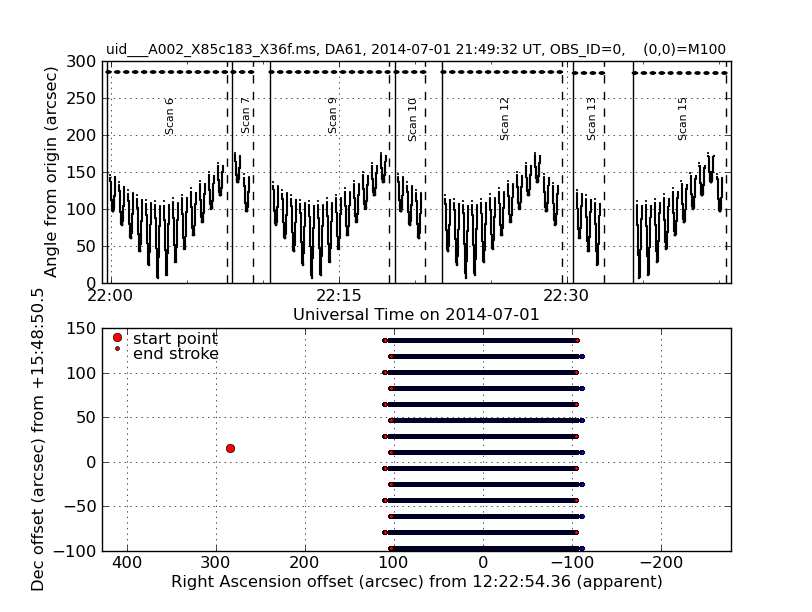
The scan pattern of the raster mapping can be visualized by issueing the following command. A plot will be shown in a window and also saved as a PNG file uid___A002_X85c183_X36f.ms.sampling.png.
<figure id="X36f.TPSampling.png">
</figure>
# In CASA
aU.getTPSampling(vis='uid___A002_X85c183_X36f.ms',
                 showplot=True,
                 plotfile='uid___A002_X85c183_X36f.ms.sampling.png')
Convert MS into Single-Dish Data Format
To calibrate the data, we need the data to be in the single-dish scantable (ASAP) format. Most of the tasks that we will use for calibration are inherited from the ASAP package, which has been incorporated into CASA. The ASAP package uses a different data format, so from a global point of view, what we are going to do is, first convert the MS to the ASAP format, then run the necessary calibration tasks, then convert the data back to the MS format. An effort for transition from ASAP to MS is ongoing; in a future version of CASA this step will become unnecessary.
We use the task sdsave to do this. The option outform, which specifies the format of the output data, is left as the default value 'ASAP'. We will split the data by antennas by using the option splitant=True.
# In CASA
sdsave(infile='uid___A002_X85c183_X36f.ms',
       splitant=True,
       outfile='uid___A002_X85c183_X36f.ms.asap',
       overwrite=True)
As three antennas were used in the observation, three corresponding ASAP datasets (uid___A002_X85c183_X36f.ms.DA61.asap, uid___A002_X85c183_X36f.ms.PM03.asap, and uid___A002_X85c183_X36f.ms.PM04.asap) are generated. As usual, we will first obtain information about the content of the datasets, using the task sdlist (which plays the same role as listobs).
# In CASA
for ant in ['DA61', 'PM03', 'PM04']:
    sdlist(infile='uid___A002_X85c183_X36f.ms.%s.asap' % ant,
           outfile='uid___A002_X85c183_X36f.ms.%s.asap.sdlist' % ant)
Here is an example of the output for uid___A002_X85c183_X36f.ms.DA61.asap. The displayed information is in principle the same as what you got from listobs (except for reduced number of antennas), although sdlist uses different expression (inherited from ASAP) from that of listobs (CASA native) -- e.g., "ScanIntent" in listobs is shown as "SrcType" in sdlist (CALIBRATE_something to CALON, ON_SOURCE to PSON, OFF_SOURCE to PSOFF, etc.), and CASA SPWs correspond to ASAP "IF"s.
# In CASA
os.system('cat uid___A002_X85c183_X36f.ms.DA61.asap.sdlist')
--------------------------------------------------------------------------------
 Scan Table Summary
--------------------------------------------------------------------------------
Project:       uid://A002/X82e287/X3
Obs Date:      2014/07/01/21:49:32
Observer:      cvlahakis
Antenna Name:  ALMA//DA61@A075
Data Records:  41726 rows
Obs. Type:     CALIBRATE_POINTING#ON_SOURCE,CALIBRATE_WVR#ON_SOURCE
Beams:         1
IFs:           25
Polarisations: 2   (linear)
Channels:      4080
Flux Unit:     K
Abscissa:      Channel
Selection:     none

Scan Source         Time range                           Int[s] Record SrcType FreqIDs MolIDs
       Beam  Position (J2000)
--------------------------------------------------------------------------------
   1 J1215+1654     2014/07/01/21:51:26.28 - 21:53:29.48   1.01574  2029  [PSON:CALON] [0, 1, 2, 3, 4, 5, 6, 7, 8] [0]
       0      J2000 12:15:03.989 +16.54.37.559
   2 J1215+1654     2014/07/01/21:55:24.90 - 21:56:25.45   0.49753  2070  [PSON:CALON, PSOFF:CALON] [0, 9, 10, 11, 12, 13, 14, 15, 16] [0]
       0      J2000 12:15:03.988 +16.54.37.560
   3 J1215+1654     2014/07/01/21:56:27.21 - 21:56:53.05   0.500364   594  [PSOFF:CALON, PSON:CALON] [0, 9, 10, 11, 12, 13, 14, 15, 16] [0]
       0      J2000 12:15:03.988 +16.54.37.561
   4 J1215+1654     2014/07/01/21:56:56.52 - 21:57:17.88   1.76957   194  [PSON:CALON] [0, 17, 18, 19, 20, 21, 22, 23, 24] [0, 1, 2, 3, 4]
       0      J2000 12:15:03.988 +16.54.37.560
   5 M100           2014/07/01/21:58:22.41 - 21:58:47.39   0.500364   594  [PSOFF:CALON, PSON:CALON] [0, 9, 10, 11, 12, 13, 14, 15, 16] [0]
       0      J2000 12:23:13.286 +15.48.50.161
   6 M100           2014/07/01/21:59:41.64 - 22:07:36.12   1.01591  7720  [PSOFF, PSON] [0, 17, 18, 19, 20, 21, 22, 23, 24] [0, 1, 2, 3, 4]
       0      J2000 12:23:13.286 +15.48.50.162
   7 M100           2014/07/01/22:07:54.69 - 22:09:19.80   1.01608  1390  [PSOFF, PSON] [0, 17, 18, 19, 20, 21, 22, 23, 24] [0, 1, 2, 3, 4]
       0      J2000 12:23:13.285 +15.48.50.164
   8 M100           2014/07/01/22:09:38.49 - 22:10:03.47   0.500364   594  [PSOFF:CALON, PSON:CALON] [0, 9, 10, 11, 12, 13, 14, 15, 16] [0]
       0      J2000 12:23:13.285 +15.48.50.165
   9 M100           2014/07/01/22:10:25.58 - 22:18:18.96   1.01586  7717  [PSOFF, PSON] [0, 17, 18, 19, 20, 21, 22, 23, 24] [0, 1, 2, 3, 4]
       0      J2000 12:23:13.285 +15.48.50.165
  10 M100           2014/07/01/22:18:38.66 - 22:20:39.48   1.01599  1965  [PSOFF, PSON] [0, 17, 18, 19, 20, 21, 22, 23, 24] [0, 1, 2, 3, 4]
       0      J2000 12:23:13.285 +15.48.50.168
  11 M100           2014/07/01/22:20:57.16 - 22:21:23.00   0.500364   594  [PSOFF:CALON, PSON:CALON] [0, 9, 10, 11, 12, 13, 14, 15, 16] [0]
       0      J2000 12:23:13.285 +15.48.50.174
  12 M100           2014/07/01/22:21:44.13 - 22:29:38.62   1.01584  7716  [PSOFF, PSON] [0, 17, 18, 19, 20, 21, 22, 23, 24] [0, 1, 2, 3, 4]
       0      J2000 12:23:13.285 +15.48.50.169
  13 M100           2014/07/01/22:30:23.68 - 22:32:24.51   1.01599  1965  [PSOFF, PSON] [0, 17, 18, 19, 20, 21, 22, 23, 24] [0, 1, 2, 3, 4]
       0      J2000 12:23:13.284 +15.48.50.173
  14 M100           2014/07/01/22:33:29.37 - 22:33:54.35   0.500364   594  [PSOFF:CALON, PSON:CALON] [0, 9, 10, 11, 12, 13, 14, 15, 16] [0]
       0      J2000 12:23:13.284 +15.48.50.175
  15 M100           2014/07/01/22:34:19.84 - 22:40:28.35   1.01584  5990  [PSOFF, PSON] [0, 17, 18, 19, 20, 21, 22, 23, 24] [0, 1, 2, 3, 4]
       0      J2000 12:23:13.284 +15.48.50.179
--------------------------------------------------------------------------------
FREQUENCIES: 9
  ID  IFNO(SPW)  #Chans  Frame   Ch0[MHz]    ChanWid[kHz]  Center[MHz]   POLNOs
   0  0               4    TOPO      183925       2500000        187675  [0]
   1  1             124    TOPO  91955.5125        -15625     90994.575  [0, 1]
   2  2               1    TOPO    90978.95      -1734375      90978.95  [0, 1]
   3  3             124    TOPO  93893.0125        -15625     92932.075  [0, 1]
   4  4               1    TOPO  92924.2625      -1937500    92924.2625  [0, 1]
   5  5             124    TOPO  102033.637         15625    102994.575  [0, 1]
   6  6               1    TOPO  102986.762       1937500    102986.762  [0, 1]
   7  7             124    TOPO  104033.637         15625    104994.575  [0, 1]
   8  8               1    TOPO  104986.762       1937500    104986.762  [0, 1]
   9  9             128    TOPO  101942.187        -15625        100950  [0, 1]
  10  10              1    TOPO  100926.562      -1781250    100926.562  [0, 1]
  11  11            128    TOPO  103757.337        -15625     102765.15  [0, 1]
  12  12              1    TOPO  102741.712      -1781250    102741.712  [0, 1]
  13  13            128    TOPO  111814.962         15625     112807.15  [0, 1]
  14  14              1    TOPO  112783.712       1781250    112783.712  [0, 1]
  15  15            128    TOPO  113689.962         15625     114682.15  [0, 1]
  16  16              1    TOPO  114658.712       1781250    114658.712  [0, 1]
  17  17           4080    TOPO   101945.85    -488.28125        100950  [0, 1]
  18  18              1    TOPO  100949.756    -1992187.5    100949.756  [0, 1]
  19  19           4080    TOPO      103761    -488.28125     102765.15  [0, 1]
  20  20              1    TOPO  102764.906    -1992187.5    102764.906  [0, 1]
  21  21           4080    TOPO    111811.3     488.28125     112807.15  [0, 1]
  22  22              1    TOPO  112806.906     1992187.5    112806.906  [0, 1]
  23  23           4080    TOPO    113686.3     488.28125     114682.15  [0, 1]
  24  24              1    TOPO  114681.906     1992187.5    114681.906  [0, 1]
--------------------------------------------------------------------------------
MOLECULES:
   ID   RestFreq          Name
    0   [] []
    1   [1.0095e+11] [Manual_window(ID=0)]
    2   [1.027941e+11] [Manual_window(ID=0)]
    3   [1.127941e+11] [Manual_window(ID=0)]
    4   [1.146691e+11] [CO_v_0_1_0(ID=3768098)]
--------------------------------------------------------------------------------
Inspect the System Noise Temperature
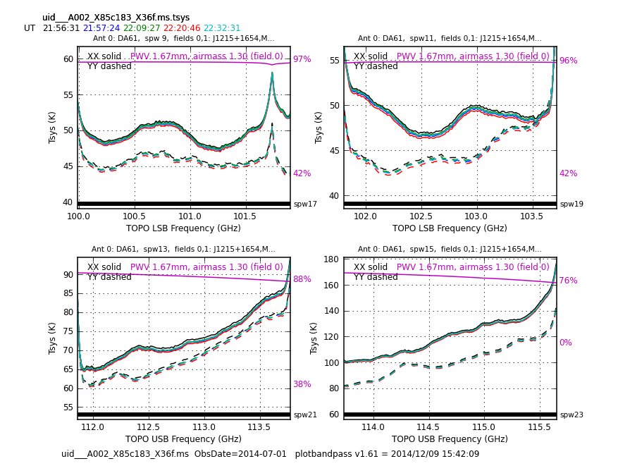
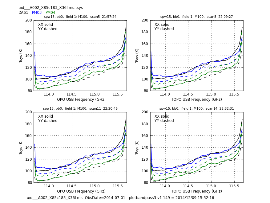
Let's start by checking the Tsys. We use the task gencal to extract the Tsys into a CASA calibration table. This table is only used for plotting and for letting CASA figure out the mapping between the science and Tsys SPW's (see "Tsys Calibration" section).
# In CASA
gencal(vis='uid___A002_X85c183_X36f.ms',
       caltable='uid___A002_X85c183_X36f.ms.tsys',
       caltype='tsys')
The generated Tsys calibration table can be plotted using the task plotbandpass and the checkCalTable function of the Analysis Utilities. The generated plots are saved in the directories uid___A002_X85c183_X36f.ms.tsys.plots.overlayTime and uid___A002_X85c183_X36f.ms.tsys.plots.
<figure id="X36f.Tsys.overlayTime.png">
</figure>
<figure id="X36f.Tsys.overlayAntenna.png.png">
</figure>
# In CASA
plotbandpass(caltable='uid___A002_X85c183_X36f.ms.tsys',
             overlay='time',
             xaxis='freq',
             yaxis='amp',
             subplot=22,
             buildpdf=False,
             interactive=False,
             showatm=True,
             pwv='auto',
             chanrange='5~123',
             showfdm=True,
             field='',
             figfile='uid___A002_X85c183_X36f.ms.tsys.plots.overlayTime/uid___A002_X85c183_X36f.ms.tsys')

es.checkCalTable('uid___A002_X85c183_X36f.ms.tsys',
                 msName='uid___A002_X85c183_X36f.ms',
                 interactive=False)
A Priori Flagging
Now we do some a-priori flagging of the edge channels. Although the "science" SPW's have 1992 MHz bandwidths with 4080 spectral channels, their edge channels are very noisy, because each intermediate frequency signal path (baseband) is equipped with a bandpass filter of ~1.8 GHz width. We flag 120 channels on each side of the "science" SPW's. As a result 3840 channels (1875 MHz bandwidth), i.e., the same number of channels and bandwidth as FDM SPW's in the 12-m array data, remain in each SPW.
# In CASA
for ant in ['DA61', 'PM03', 'PM04']:
    sdflag(infile='uid___A002_X85c183_X36f.ms.%s.asap' % ant,
           mode='manual',
           spw='17:0~119;3960~4079,19:0~119;3960~4079,21:0~119;3960~4079,23:0~119;3960~4079',
           overwrite = True)
Tsys Calibration
We calibrate the data into brightness temperature in units of K, using the equation Ta* = Tsys*(ON-OFF)/OFF, where ON and OFF are the data on-source (i.e., during the raster scanning) and off-source (on a reference position where only background emission exists), respectively. The calibration is done by the task Template:Sdcal2. It requires the list of the "science" SPW's and Tsys SPW's, and the correspondence between them. We can tell from the listobs (or sdlist) output that Tsys SPW's 9, 11, 13, and 15 correspond to "science" SPW's 17, 19, 21, and 23, respectively; but the function tsysspwmap helps to map Tsys SPW's to science SPW's in an automated way:
# In CASA
from recipes.almahelpers import tsysspwmap
tsysmap = tsysspwmap(vis='uid___A002_X85c183_X36f.ms',
                     tsystable='uid___A002_X85c183_X36f.ms.tsys')
The obtained variable tsysmap is a list which looks like as follows. The N-th (counted from 0) item indicates the Tsys SPW corresponding to the SPW ID N, e.g., the 23rd item is 15, thus the Tsys SPW 15 corresponds to the science SPW 23.
[0, 1, 2, 3, 4, 5, 6, 7, 8, 9, 9, 11, 11, 13, 13, 15, 15, 9, 9, 11, 11, 13, 13, 15, 15]
Now this information needs to be translated into a dictionary variable which Template:Sdcal2 requires. The mapping between the science SPW's (17, 19, 21, and 23) and Tsys SPW's is given by the following piece of code:
# In CASA
spwmap = {}
for i in [17, 19, 21, 23]:
    if not tsysmap[i] in spwmap.keys():
        spwmap[tsysmap[i]] = []
    spwmap[tsysmap[i]].append(i)
The obtained correspondence between Tsys and science SPW's is stored in the dictionary spwmap which looks like the following:
{9: [17], 11: [19], 13: [21], 15: [23]}
This is given to sdcal2, along with the comma-separated lists of SPW's. An important parameter of the task is calmode. In case of the science dataset uid___A002_X85c183_X36f, calmode should be set to 'ps,tsys,apply'. 'ps' means that the data at dedicated reference position are used as "OFF" for the OFF subtraction, (ON-OFF)/OFF. 'tsys' is to calibrate the data using Tsys. 'apply' is to apply both calibrations above (OFF-subtraction and Tsys).
# In CASA
for ant in ['DA61', 'PM03', 'PM04']:
    sdcal2(infile='uid___A002_X85c183_X36f.ms.%s.asap' % ant,
           calmode='ps,tsys,apply',
           spw='9,11,13,15,17,19,21,23',
           tsysspw='9,11,13,15',
           spwmap=spwmap,
           outfile='uid___A002_X85c183_X36f.ms.%s.asap.cal' % ant,
           overwrite=True)
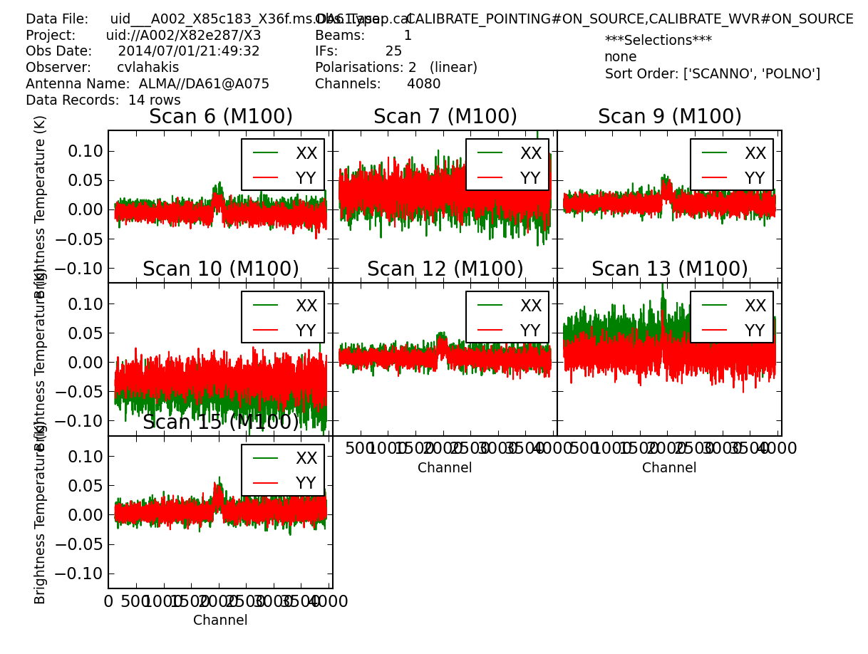
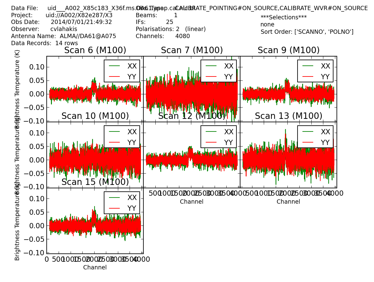
A new ASAP dataset with additional suffix '.cal' is generated for each antenna. Before proceeding to the next step, we can plot the calibrated spectra using the SDcheckSpectra function of the Analysis Utilities. PNG files will be created in, e.g., uid___A002_X85c183_X36f.ms.DA61.asap.cal.plots directory. You will find the CO line in SPW 23 of the science datasets.
<figure id="X36f.spw23.cal.png">
</figure>
# In CASA
for ant in ['DA61', 'PM03', 'PM04']:
    es.SDcheckSpectra('uid___A002_X85c183_X36f.ms.%s.asap.cal' % ant,
                      spwIds='17,19,21,23',
                      interactive=False)
Note: For amplitude calibrator datasets, (as opposed to science target maps) the calmode option for sdcal2 should be 'otfraster,tsys,apply' ('otfraster' instead of 'ps'). 'otfraster' tells the task to use both ends of each raster row as "OFF" data (as opposed to a dedicated "OFF" sky measurement). This is because temporal fluctuation of atmospheric emission is the dominant source of noise in radio continuum observations, and hence the "OFF" needs to be as close as possible to the "ON" in time (and spatial location).
Application of Non-Linearity Correction Factor
In the period of Early Science Cycle 1/2, single-dish data taken with the ACA correlator suffer from non-linearity which originates in the digital signal processing. Its impact was thoroughly studied both experimentally and theoretically, and it was concluded that multiplication by a correction factor of 1.25 yields an amplitude accuracy of +/-5%. This correction is done by the task sdscale. A new ASAP dataset with additional suffix '.nlc' (for Non-Linearity Correction) will be created for each antenna.
# In CASA
for ant in ['DA61', 'PM03', 'PM04']:
    sdscale(infile='uid___A002_X85c183_X36f.ms.%s.asap.cal' % ant,
            outfile='uid___A002_X85c183_X36f.ms.%s.asap.cal.nlc' % ant,
            factor=1.25)
An upgrade of the ACA correlator hardware and software is expected to solve the non-linearity issue. Thus this step will become unnecessary for data taken in the near future.
Baseline Subtraction (only for Science Datasets)
Note: this step is appropriate for spectral line observations (science datasets) but should not be done for the continuum observations (amplitude calibrator datasets) -- it would eliminate the continuum emission!
We will subtract spectral baselines using the task sdbaseline.
A tweak (removing flagged rows) is needed before proceeding, to avoid an issue in CASA 4.3 (which will be fixed in CASA 4.4).
# In CASA
for ant in ['DA61', 'PM03', 'PM04']:
    tb.open('uid___A002_X85c183_X36f.ms.%s.asap.cal.nlc' % ant, nomodify=False)
    flaggedrows = tb.query('FLAGROW==1').rownumbers()
    if len(flaggedrows) > 0: tb.removerows(flaggedrows)
    tb.flush()
    tb.close()
Now we are ready to execute sdbaseline. With the option "maskmode='auto'", the task automatically finds line features from individual spectra and excludes them from baseline fitting. A caveat is that the line finding may not work very well in some cases, including this dataset (see "Subtract a Residual Background from the Image" section below).
# In CASA
for ant in ['DA61', 'PM03', 'PM04']:
    sdbaseline(infile='uid___A002_X85c183_X36f.ms.%s.asap.cal.nlc' % ant,
               spw='17,19,21,23',
               maskmode='auto',
               thresh=5.0,
               avg_limit=4,
               blfunc='poly',
               order=1,
               outfile='uid___A002_X85c183_X36f.ms.%s.asap.cal.nlc.bl' % ant,
               overwrite=True)
Datasets with yet another suffix ".bl" are generated. The spectra can be checked using SDcheckSpectra which we have already used in a previous step.
<figure id="X36f.spw23.cal.bl.png">
</figure>
# In CASA
for ant in ['DA61', 'PM03', 'PM04']:
    es.SDcheckSpectra('uid___A002_X85c183_X36f.ms.%s.asap.cal.nlc.bl' % ant,
                      spwIds='17,19,21,23',
                      interactive=False)
Convert Single-Dish Data back to MS Format
Now the calibrated data need to be coverted back to the CASA MS format, because the imaging task (sdimaging) only accepts MS. The CASA task sdsave will do this.
# In CASA
for ant in ['DA61', 'PM03', 'PM04']:
    sdsave(infile='uid___A002_X85c183_X36f.ms.%s.asap.cal.nlc.bl' % ant,
           outfile='uid___A002_X85c183_X36f.ms.%s.asap.cal.nlc.bl.ms' % ant,
           spw='17,19,21,23',
           outform='MS2')
And concatenate the data which were split by antennas, using the task concat.
# In CASA
concat(vis=['uid___A002_X85c183_X36f.ms.DA61.asap.cal.nlc.bl.ms',
            'uid___A002_X85c183_X36f.ms.PM03.asap.cal.nlc.bl.ms',
            'uid___A002_X85c183_X36f.ms.PM04.asap.cal.nlc.bl.ms'],
       concatvis='uid___A002_X85c183_X36f.ms.cal')
We do not concatenate separate Execution Blocks, because we need to determine and apply day-by-day Jy/K conversion factor.
Note that one of the antennas, PM02, had a problem in the first baseband (SPW 17) on 2014-07-05, and its impact may not be specific to this one SPW (e.g., it may have resulted in poor pointing calibration). Therefore the PM02 data should be excluded from the concatenation for the affected datasets: uid___A002_X8602fa_Xc3 (amplitude calibrator), uid___A002_X8602fa_X2ab (science), and uid___A002_X8602fa_X577 (science).
Optionally Image the Amplitude Calibrator and Measure the Value of Jy/K
At this stage you should have run all 9 science datasets through their respective scriptForSDCalibration.py, i.e., all 9 datasets have been calibrated into units of Kelvins. The next step is to apply Jy/K conversion factors that have been derived from observations of an amplitude calibrator (one Jy/K value determined per day and per SPW). The resulting Jy/K values are given at the end of this section.
If you want to know details of how the Jy/K values are determined, a summary is given below. Otherwise, you can skip ahead to the next section M100_Band3_SingleDish_4.3#Convert the Science Target Units from Kelvin to Jansky to continue the calibration.
Determination of the Jy/K conversion factor is achieved by imaging a source whose continuum flux is known and measuring the observed brightness temperature. One observation of this source - the amplitude calibrator - was made per day, giving a total of four datasets:
#Amplitude Calibrator
uid___A002_X85c183_X895      Observed from 2014-07-01T23:35:23.1 to 2014-07-02T00:07:54.6 (UTC)      DA61, PM03, PM04
uid___A002_X8602fa_Xc3       Observed from 2014-07-05T23:21:25.6 to 2014-07-05T23:53:41.0 (UTC)      PM02, PM03, PM04
uid___A002_X864236_Xe1       Observed from 2014-07-07T22:27:35.4 to 2014-07-07T23:01:05.7 (UTC)      PM03, PM04
uid___A002_X86fcfa_X3ae      Observed from 2014-07-17T21:48:30.0 to 2014-07-17T22:20:52.2 (UTC)      DV10, PM03, PM04
The true size of the beam (point spread function), on which the Jy/K value depends, in a map is determined be several ingredients.
- The intrinsic beam size is determined by the antenna diameter and optics (and of course wavelength). Here we assume the intrinsic beam size of 1.13*lambda/D, where D=12 [m] is the diameter of the antennas, and the factor 1.13 is derived from the optics design of the ALMA 12-m antennas.
- The effective beam size is broadened by the following causes:
- The scanning pattern used to observe the map (i.e., sample spacing in both directions).
- The method used to grid the individual spectra into a map/cube.
The Analysis Utilities provides several tools to get estimates of these.
If you wish to try this out for yourself, you will first need to download the raw amplitude calibrator data file M100_Band3_TP_ampcal_UncalibratedData.tgz. How to obtain the data is described at M100_Band3#Obtaining the Data. Once you have unpacked the data you will have a directory called M100_Band3_TP_ampcal_UncalibratedData. In this directory, execute the script "ScriptForImagingAmpCalAndDerivingJyPerK.py" to calibrate all four calibrator datasets using for-loops (run execfile('ScriptForImagingAmpCalAndDerivingJyPerK.py') in CASA).
The resulting Jy/K values are as follows. Note that the values for individual antennas are averaged for each day, each SPW, because the antennas used for the Science observations were not necessarily available for the corresponding amplitude calibrator observations.
#Date        Amp_Cal_Dataset           SPW17   SPW19   SPW21   SPW23
2014-07-01   uid___A002_X85c183_X895   41.37   42.39   43.45   42.82
2014-07-05   uid___A002_X8602fa_Xc3    40.99   42.74   40.08   42.09
2014-07-07   uid___A002_X864236_Xe1    39.42   42.08   40.18   40.82
2014-07-17   uid___A002_X86fcfa_X3ae   43.49   43.70   42.01   43.04
Convert the Science Target Units from Kelvin to Jansky
The science data, which have been calibrated into brightness temperature in units of K, are now converted into Jy units by multiplying the Jy/K factors derived above. This step is done by the script "ScriptForJyPerKConversion.py" (run execfile('ScriptForJyPerKConversion.py') in CASA).
Define the lists of SPWs and corresponding Jy/K factors to process the data using for-loops.
# In CASA

# List the science spws
spwlist = [17, 19, 21, 23]

# List the Jy/K values (corresponding to the list of the science spws above)
# that were the output from ScriptForImagingAmpCalAndDerivingJyPerK.py
jyperklist0701 = [41.37, 42.39, 43.45, 42.82]
jyperklist0705 = [40.99, 42.74, 40.08, 42.09]
jyperklist0707 = [39.42, 42.08, 40.18, 40.82]
jyperklist0717 = [43.49, 43.70, 42.01, 43.04]
Make a copy of calibrated dataset, with an additional suffix ".jy", and multiply the Jy/K value for each SPW. This is done by the scaleAutocorr function of Analysis Utilities.
# In CASA

# Data taken on 2014-07-01
for name in ['uid___A002_X85c183_X36f', 'uid___A002_X85c183_X60b']:
    os.system('rm -Rf %s.ms.cal.jy' % name)
    os.system('cp -Rf %s.ms.cal %s.ms.cal.jy' % (name, name))
    for (spw, jyperk) in zip(spwlist, jyperklist0701):
        aU.scaleAutocorr(vis='%s.ms.cal.jy' % name, scale=jyperk, spw=spw)

# Data taken on 2014-07-05
for name in ['uid___A002_X8602fa_X2ab', 'uid___A002_X8602fa_X577']:
    os.system('rm -Rf %s.ms.cal.jy' % name)
    os.system('cp -Rf %s.ms.cal %s.ms.cal.jy' % (name, name))
    for (spw, jyperk) in zip(spwlist, jyperklist0705):
        aU.scaleAutocorr(vis='%s.ms.cal.jy' % name, scale=jyperk, spw=spw)

# Data taken on 2014-07-07
for name in ['uid___A002_X864236_X2d4', 'uid___A002_X864236_X693']:
    os.system('rm -Rf %s.ms.cal.jy' % name)
    os.system('cp -Rf %s.ms.cal %s.ms.cal.jy' % (name, name))
    for (spw, jyperk) in zip(spwlist, jyperklist0707):
        aU.scaleAutocorr(vis='%s.ms.cal.jy' % name, scale=jyperk, spw=spw)

# Data taken on 2014-07-17
for name in ['uid___A002_X86fcfa_Xd9', 'uid___A002_X86fcfa_X664',
    'uid___A002_X86fcfa_X96c']:
    os.system('rm -Rf %s.ms.cal.jy' % name)
    os.system('cp -Rf %s.ms.cal %s.ms.cal.jy' % (name, name))
    for (spw, jyperk) in zip(spwlist, jyperklist0717):
        aU.scaleAutocorr(vis='%s.ms.cal.jy' % name, scale=jyperk, spw=spw)
Image the Science Target
Now all the science datasets have been calibrated into Jy units. The next (final) step is to image the science data. This step is done by the script "ScriptForImagingScienceTarget.py" (run execfile('ScriptForImagingScienceTarget.py') in CASA).
Define the list of the calibrated science datasets, which the CASA task sdimaging accepts.
# In CASA
sciencedata = [('%s.ms.cal.jy' % name) for name in basename_science]
Obtain the data sampling and determine the cell spacing and map size based on the mean frequency of the target SPW. This part is in principle the same as the corresponding procedure in the "Image the Amplitude Calibrator and Measure the Value of Jy/K" section.
# In CASA
fwhmfactor = 1.13
diameter = 12

xSampling, ySampling, maxsize = aU.getTPSampling(sciencedata[0], showplot=False)

spw = 23

msmd.open(sciencedata[0])
freq = msmd.meanfreq(spw)
msmd.close()
print "SPW %d: %.3f GHz" % (spw, freq*1e-9)

theorybeam = aU.primaryBeamArcsec(frequency=freq*1e-9,
                                  fwhmfactor=fwhmfactor,
                                  diameter=diameter)

cell = theorybeam/9.0
imsize = int(round(maxsize/cell)*2)
Now the data are imaged. The velocity channel maps of the CO J=1-0 line (restfreq='115.271201800GHz') are created as a data cube which covers the velocity range of 1400-1700 km/s at a spacing of 5 km/s (start='1400km/s', width='5km/s', nchan=70).
Note: The Jy/K value depends on the parameters of gridding convolution (i.e., "gridfunction", "cell", and function-specific parameters ["convsupport" for gridfunction='SF']). That is, the same gridding parameters should be used for both amplitude calibrator and science images -- otherwise the calibration into Jy unit becomes invalid.
# In CASA
sdimaging(infiles=sciencedata,
          field='M100',
          spw='%d' % spw,  #sciencespw
          nchan=70,
          mode='velocity',
          start='1400km/s',
          width='5km/s',
          veltype='radio',
          outframe='lsrk',
          restfreq='115.271201800GHz',
          gridfunction='SF',
          convsupport=6,
          stokes='',
          phasecenter='J2000 12h22m54.9 +15d49m15',
          ephemsrcname='',
          imsize=imsize,
          cell=str(cell)+'arcsec',
          overwrite=True,
          outfile='M100_TP_CO_cube.image')
The produced image has the brightness unit of K in the image header, which is not correct. Modify the header using the task imhead.
# In CASA
imhead(imagename='M100_TP_CO_cube.image',
       mode='put',
       hdkey='bunit',
       hdvalue='Jy/beam')
(Optionally) Subtract a Residual Background from the Image
Now you can browse the data cube using the viewer.
# In CASA
viewer('M100_TP_CO_cube.image')
If you plot the line profile using the viewer, you may notice that the background (i.e., line-free channels) level is slightly negative. To correct this, spectral baselines are subtracted from the image using the task imcontsub.
# In CASA
imcontsub(imagename='M100_TP_CO_cube.image',
          linefile='M100_TP_CO_cube.bl.image',
          contfile='M100.ignorethis.image',
          fitorder=1,
          chans='0~7;62~69')
os.system('rm -rf M100.ignorethis.image')
The main cause of the negative baseline is the following. The task sdbaseline with maskmode='auto' is supposed to find lines from the data and exclude the detected lines from baseline fitting. However, the CO line from M100 is not bright enough to be detected from individual spectra (1-s integration), and hence sdbaseline included the velocity ranges of the line into baseline fitting. The impact of this effect would be smaller if the line is brighter, or narrower w.r.t. the correlator bandwidth.
Add Restoring Beam Header Information to the Science Image
The image does not have the beam size, which is necessary for combining the image with interferometric data, in the header. The beam size (including the broadening due to gridding convolution and data sampling) is calculated using the function sfBeam of the Analysis Utilities and then written into the header using the functions of the ia tool.
# In CASA
minor, major, fwhmsfBeam, sfBeam = aU.sfBeam(frequency=freq*1e-9,
        pixelsize=cell,
        convsupport=6,
        img=None, #to use Gaussian theorybeam
        stokes='both',
        xSamplingArcsec=xSampling,
        ySamplingArcsec=ySampling,
        fwhmfactor=fwhmfactor,
        diameter=diameter)

ia.open('M100_TP_CO_cube.bl.image')
ia.setrestoringbeam(major=str(sfBeam)+'arcsec', minor=str(sfBeam)+'arcsec', pa='0deg')
ia.done()
Quick Look at the Results
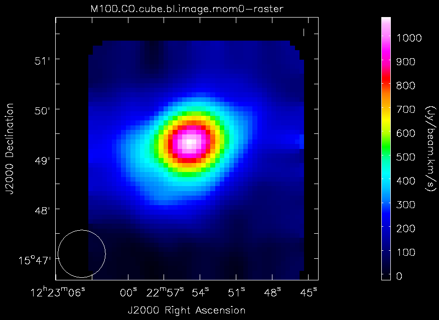
Make a 0th moment (integrated intensity) map using the task immoments and browse it using the viewer.
<figure id="M100.CO.cube.bl.image.mom0.png">
</figure>
# In CASA
os.system('rm -rf *M100_TP_CO_cube.bl.image.mom0')
immoments(imagename='M100_TP_CO_cube.bl.image',
          moments=[0],
          axis='spectral',
          chans='8~61',
          outfile='M100_TP_CO_cube.bl.image.mom0')

viewer('M100_TP_CO_cube.bl.image.mom0')
Combination with 12m and 7m Array Data
If you wish to learn how to combine the Total Power data with interferometric 12m and 7m data, see the guide for Data Combination M100_Band3_Combine_4.3
Last checked on CASA Version 4.3.0.