DataWeightsAndCombination

This page is currently under construction.

Description of CASA Weights

A memo describing weights in CASA can be found at http://casa.nrao.edu/Memos/CASA-data-weights.pdf

Concat with 1/sigma² scaling of Weights

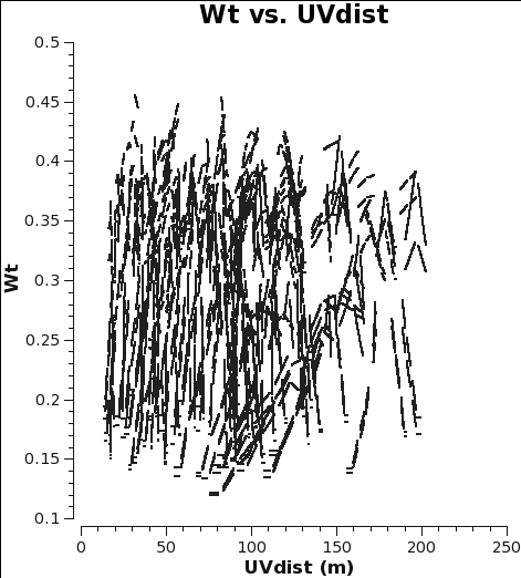
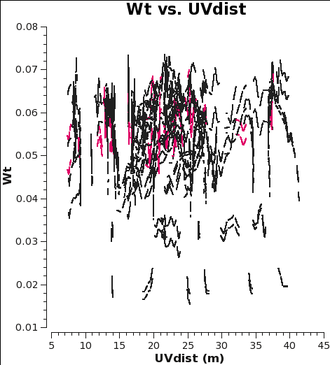
<figure id="7m_WT.png">

12m weights.

</figure>

<figure id="12m_WT.png">

7m weights.

</figure>

When combining data with disparate properties it is very important that the relative weights of each visibility be in the correct proportion to the other data according to the radiometer equation. Formally, the visibility weights should be proportional to 1/sigma**2 where sigma is the variance or rms noise of a given visibility.

In CASA 4.2.1 and earlier, the data weights are 1 upon import, later in the standard calibration procedure, applycal scales the weights by 1/[(Tsys(i) * Tsys(j)] if calwt=True for the Tsys table applycal. As an example, we plot the weights of 7m and 12m data imported in CASA 4.2.1. No averaging can be turned on when plotting the weights.

# In CASA
os.system('rm -rf 7m_WT.png 12m_WT.png')
plotms(vis='m100_12m_CO.ms',yaxis='wt',xaxis='uvdist',spw='0~2:200',
       coloraxis='spw',plotfile='12m_WT.png')
#
plotms(vis='m100_7m_CO.ms',yaxis='wt',xaxis='uvdist',spw='0~2:200',
       coloraxis='spw',plotfile='7m_WT.png')

As you can see from these plots, the weights are quite similar at this stage because the data were taken under similar weather conditions and hence Tsys.

Assuming that the 7m and 12m antennas have similar apperture and quantization efficiencies (a reasonable assumption since they were designed this way), the rms noise in a single channel for a single visibility is:

[math]\displaystyle{ \sigma_{ij}=\frac{2k}{A_{eff}} }[/math] [math]\displaystyle{ \sqrt{\frac{T_{sys,i} T_{sys,j}}{\Delta\nu_{ch} t_{ij}}} }[/math]

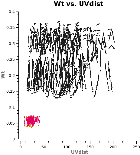
<figure id="Intcombo_0.193_WT.png">

7m and 12m weights after scaling by relative sensitivity.

</figure>

Where k is Boltzmann's constant, A_eff is the effective antenna area, T_sys,i is the system temperature for antenna i, Δν_ch is the channel width, and t_ij is the integration time per visibility.

The two key things that are different between the 7m and 12m-array data are that the effective dish Areas are different by (7/12)² and the integration times are different by sqrt(10.1/6.05). Since dish area is in the numerator of the radiometer equation and integration time per visibility is in the denominator, and assuming WT propto 1/sigma², the 7m weight should be scaled by: (7./12.)⁴ x (10.1/6.05) = 0.193 to account for the difference in telescope size and integration time per visibility.

# In CASA
# Concat and scale weights
os.system('rm -rf M100_Intcombo_0.193.ms')
concat(vis=['m100_12m_CO.ms','m100_7m_CO.ms'],
       concatvis='M100_Intcombo_0.193.ms',
       visweightscale=[1,0.193])

Now plot the concatenated weights to verify they are as expected.

# In CASA
os.system('rm -rf Intcombo_0.193_WT.png')
plotms(vis='M100_Intcombo_0.193.ms',yaxis='wt',xaxis='uvdist',spw='0~2:200',
       coloraxis='spw',plotfile='Intcombo_0.193_WT.png')

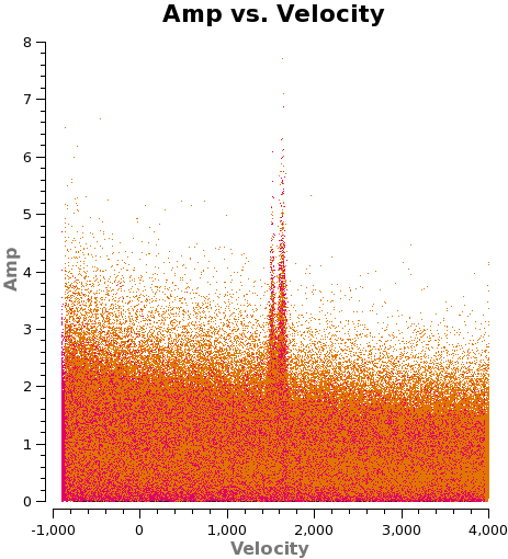
<figure id="M100_Intcombo_0.193_vel.png">

Amplitude as a function of velocity.

</figure>