Calibrating an EVLA OSRO HI data set
Overview
Currently, this describes the reduction of the Leo Ring dataset collected with WIDAR0. This page will need to be revised when "real" OSRO data are acquired.
Importing Data
importing data will probably be quirky; let's not discuss the details of this yet.
Get Some Basic Information on The Data
Use listobs (roughly equivalent to LISTR in AIPS) to list information about the dataset's scans, correlator setup, and antenna positions.
#  listobs :: List data set summary in the logger
vis                 = 'leotest.ms'      #  Name of input visibility file (MS)
verbose             =       True
async               =      False        #  If true the taskname must be started using
                                        #   listobs(...)
will produce output that looks like this:
2010-02-11 18:11:34 INFO listobs	##########################################
2010-02-11 18:11:34 INFO listobs	##### Begin Task: listobs            #####
2010-02-11 18:11:34 INFO  	listobs::::casa
2010-02-11 18:11:34 INFO listobs	================================================================================
2010-02-11 18:11:34 INFO listobs	           MeasurementSet Name:  /export/home/rso-lchomiuk/test/Leo/leotest.ms      MS Version 2
2010-02-11 18:11:34 INFO listobs	================================================================================
2010-02-11 18:11:34 INFO listobs	   Observer: leo2pt     Project: T.B.D.
2010-02-11 18:11:34 INFO listobs	Observation: VLA
2010-02-11 18:11:34 INFO listobs	Data records: 70290       Total integration time = 11264.5 seconds
2010-02-11 18:11:34 INFO listobs	   Observed from   18-Dec-2009/10:52:17.0   to   18-Dec-2009/14:00:01.5 (UTC)
2010-02-11 18:11:35 INFO  	listobs::ms::summary
2010-02-11 18:11:35 INFO listobs	   ObservationID = 0         ArrayID = 0
2010-02-11 18:11:35 INFO listobs	  Date        Timerange (UTC)          Scan  FldId FieldName    nVis   Int(s)   SpwIds
2010-02-11 18:11:35 INFO listobs	  18-Dec-2009/10:52:17.0 - 10:53:45.0     1      0 J1042+1203   660    9.6      [0]
2010-02-11 18:11:35 INFO listobs	              10:54:14.0 - 10:56:51.5     2      1 J1042+1203   1122   9.71     [0]
2010-02-11 18:11:35 INFO listobs	              10:57:20.0 - 11:06:57.5     3      2 Leo-1        3894   9.92     [0]
2010-02-11 18:11:35 INFO listobs	              11:07:25.0 - 11:17:03.0     4      3 Leo-2        3894   9.93     [0]
2010-02-11 18:11:35 INFO listobs	              11:17:32.0 - 11:22:10.0     5      2 Leo-1        1914   9.86     [0]
2010-02-11 18:11:35 INFO listobs	              11:22:39.0 - 11:27:16.5     6      3 Leo-2        1914   9.83     [0]
2010-02-11 18:11:35 INFO listobs	              11:27:45.0 - 11:30:23.5     7      1 J1042+1203   1122   9.82     [0]
2010-02-11 18:11:35 INFO listobs	              11:30:52.0 - 11:40:30.0     8      2 Leo-1        3894   9.93     [0]
2010-02-11 18:11:35 INFO listobs	              11:40:59.0 - 11:50:36.5     9      3 Leo-2        3894   9.92     [0]
2010-02-11 18:11:35 INFO listobs	              11:51:05.0 - 11:55:42.5    10      2 Leo-1        1914   9.83     [0]
2010-02-11 18:11:35 INFO listobs	              11:56:11.0 - 12:00:49.0    11      3 Leo-2        1914   9.86     [0]
2010-02-11 18:11:35 INFO listobs	              12:01:18.0 - 12:03:56.0    12      1 J1042+1203   1122   9.76     [0]
2010-02-11 18:11:35 INFO listobs	              12:04:25.0 - 12:14:03.0    13      2 Leo-1        3894   9.93     [0]
2010-02-11 18:11:35 INFO listobs	              12:14:32.0 - 12:24:09.0    14      3 Leo-2        3894   9.9      [0]
2010-02-11 18:11:35 INFO listobs	              12:24:37.0 - 12:29:15.0    15      2 Leo-1        1914   9.86     [0]
2010-02-11 18:11:35 INFO listobs	              12:29:44.0 - 12:34:21.5    16      3 Leo-2        1914   9.83     [0]
2010-02-11 18:11:35 INFO listobs	              12:34:49.0 - 12:37:28.0    17      1 J1042+1203   1122   9.88     [0]
2010-02-11 18:11:35 INFO listobs	              12:37:57.0 - 12:47:35.0    18      2 Leo-1        3894   9.93     [0]
2010-02-11 18:11:35 INFO listobs	              12:48:04.0 - 12:57:41.5    19      3 Leo-2        3894   9.92     [0]
2010-02-11 18:11:35 INFO listobs	              12:58:10.0 - 13:02:48.0    20      2 Leo-1        1914   9.86     [0]
2010-02-11 18:11:35 INFO listobs	              13:03:17.0 - 13:07:54.5    21      3 Leo-2        1914   9.83     [0]
2010-02-11 18:11:35 INFO listobs	              13:08:23.0 - 13:11:01.5    22      1 J1042+1203   1122   9.82     [0]
2010-02-11 18:11:35 INFO listobs	              13:11:31.0 - 13:21:08.5    23      2 Leo-1        3894   9.92     [0]
2010-02-11 18:11:35 INFO listobs	              13:21:37.0 - 13:31:14.5    24      3 Leo-2        3894   9.92     [0]
2010-02-11 18:11:35 INFO listobs	              13:31:43.0 - 13:36:21.0    25      2 Leo-1        1914   9.86     [0]
2010-02-11 18:11:35 INFO listobs	              13:36:50.0 - 13:41:27.5    26      3 Leo-2        1914   9.83     [0]
2010-02-11 18:11:35 INFO listobs	              13:41:56.0 - 13:44:34.5    27      1 J1042+1203   1122   9.82     [0]
2010-02-11 18:11:35 INFO listobs	              13:48:02.0 - 14:00:01.5    28      4 1331+305     4818   9.99     [0]
2010-02-11 18:11:35 INFO listobs	           (nVis = Total number of time/baseline visibilities per scan)
2010-02-11 18:11:35 INFO listobs	Fields: 5
2010-02-11 18:11:35 INFO listobs	  ID   Code Name         RA            Decl           Epoch   SrcId nVis
2010-02-11 18:11:35 INFO listobs	  0    NONE J1042+1203   10:42:44.6052 +12.03.31.2641 J2000   0     660
2010-02-11 18:11:35 INFO listobs	  1    D    J1042+1203   10:42:44.6052 +12.03.31.2641 J2000   1     6732
2010-02-11 18:11:35 INFO listobs	  2    NONE Leo-1        10:47:22.0000 +12.16.38.0000 J2000   2     29040
2010-02-11 18:11:35 INFO listobs	  3    NONE Leo-2        10:46:45.0000 +11.50.38.0000 J2000   3     29040
2010-02-11 18:11:35 INFO listobs	  4    K    1331+305     13:31:08.2880 +30.30.32.9589 J2000   4     4818
2010-02-11 18:11:35 INFO listobs	   (nVis = Total number of time/baseline visibilities per field)
2010-02-11 18:11:35 INFO listobs	Spectral Windows:  (1 unique spectral windows and 1 unique polarization setups)
2010-02-11 18:11:35 INFO listobs	  SpwID  #Chans Frame Ch1(MHz)    ChanWid(kHz)TotBW(kHz)  Ref(MHz)    Corrs
2010-02-11 18:11:35 INFO listobs	  0         256 TOPO  1415.3756   7.8125      2000        1415.3756   RR  LL
2010-02-11 18:11:35 INFO listobs	Sources: 6
2010-02-11 18:11:35 INFO listobs	  ID   Name         SpwId RestFreq(MHz)  SysVel(km/s)
2010-02-11 18:11:35 INFO listobs	  0    J1042+1203   0     -              -
2010-02-11 18:11:35 INFO listobs	  1    J1042+1203   0     -              -
2010-02-11 18:11:35 INFO listobs	  2    Leo-1        0     -              -
2010-02-11 18:11:35 INFO listobs	  3    Leo-2        0     -              -
2010-02-11 18:11:35 INFO listobs	  4    J1331+3030   0     -              -
2010-02-11 18:11:35 INFO listobs	  5    J1331+3030   0     -              -
2010-02-11 18:11:35 INFO listobs	Antennas: 12:
2010-02-11 18:11:35 INFO listobs	  ID   Name  Station   Diam.    Long.         Lat.
2010-02-11 18:11:35 INFO listobs	  0    ea02  E02       25.0 m   -107.37.04.4  +33.54.01.1
2010-02-11 18:11:35 INFO listobs	  1    ea03  E09       25.0 m   -107.36.45.1  +33.53.53.6
2010-02-11 18:11:35 INFO listobs	  2    ea04  W01       25.0 m   -107.37.05.9  +33.54.00.5
2010-02-11 18:11:35 INFO listobs	  3    ea05  W08       25.0 m   -107.37.21.6  +33.53.53.0
2010-02-11 18:11:35 INFO listobs	  4    ea08  N01       25.0 m   -107.37.06.0  +33.54.01.8
2010-02-11 18:11:35 INFO listobs	  5    ea09  E06       25.0 m   -107.36.55.6  +33.53.57.7
2010-02-11 18:11:35 INFO listobs	  6    ea15  W06       25.0 m   -107.37.15.6  +33.53.56.4
2010-02-11 18:11:35 INFO listobs	  7    ea19  W04       25.0 m   -107.37.10.8  +33.53.59.1
2010-02-11 18:11:35 INFO listobs	  8    ea24  W05       25.0 m   -107.37.13.0  +33.53.57.8
2010-02-11 18:11:35 INFO listobs	  9    ea25  N02       25.0 m   -107.37.06.2  +33.54.03.5
2010-02-11 18:11:35 INFO listobs	  10   ea27  E03       25.0 m   -107.37.02.8  +33.54.00.5
2010-02-11 18:11:35 INFO listobs	  11   ea28  N08       25.0 m   -107.37.07.5  +33.54.15.8
2010-02-11 18:11:35 INFO  	listobs::::casa
2010-02-11 18:11:35 INFO listobs	##### End Task: listobs              #####
2010-02-11 18:11:35 INFO listobs	##########################################
Some things to note here are: The phase calibrator is called J1042+1203, the flux calibrator is 1331+305, and there are two science pointings, Leo-1 and Leo-2. The correlator is set up in such a way to have one spectral window (or IF). This window is sampled with 256 channels each 7.8 kHz wide. There are no cross-polarization data (note that 'Corrs' is set to only 'RR LL').
Choose a Reference Antenna
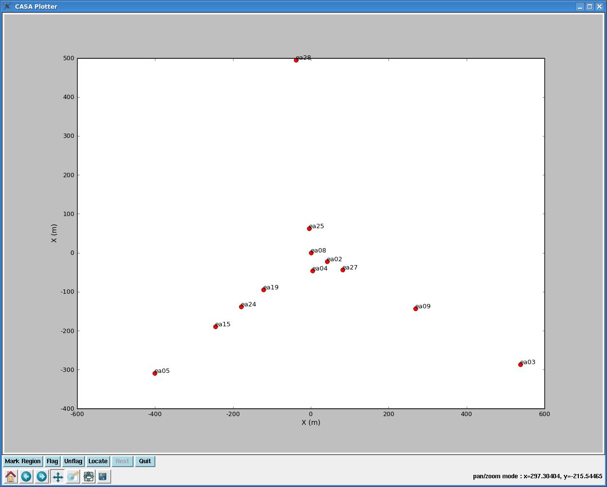
We'd like our reference antenna to be near the center of the array, and the easiest way to envision the array layout is with plotants.
#  plotants :: Plot the antenna distribution in the local reference frame:
vis                 = 'leotest.ms'      #  Name of input visibility file (MS)
figfile             =         ''        #  Save the plotted figure to this file
async               =      False        #  If true the taskname must be started using
                                        #   plotants(...)
will produce a plot that looks like this:
You can zoom and pan if you click on this icon: ![]() . Then, holding down your left mouse button and fiddling with the mouse will let you pan; holding down the right mouse button and fiddling with the mouse enables zooming in and out. Make note of an antenna near the center of the array, and check the observing logs to make sure nothing fishy happened to it during the observations. You can also take a quick look at the antenna in plotms to make sure it looks reasonably steady (check out this tutorial for an introduction to plotms).
. Then, holding down your left mouse button and fiddling with the mouse will let you pan; holding down the right mouse button and fiddling with the mouse enables zooming in and out. Make note of an antenna near the center of the array, and check the observing logs to make sure nothing fishy happened to it during the observations. You can also take a quick look at the antenna in plotms to make sure it looks reasonably steady (check out this tutorial for an introduction to plotms).
Here, we choose antenna EA25. When giving this antenna as an input to calibration routines, it can be referred to in several ways: 'ea25', '9', or 'N02' (see the output from listobs).
First Round of Data Flagging
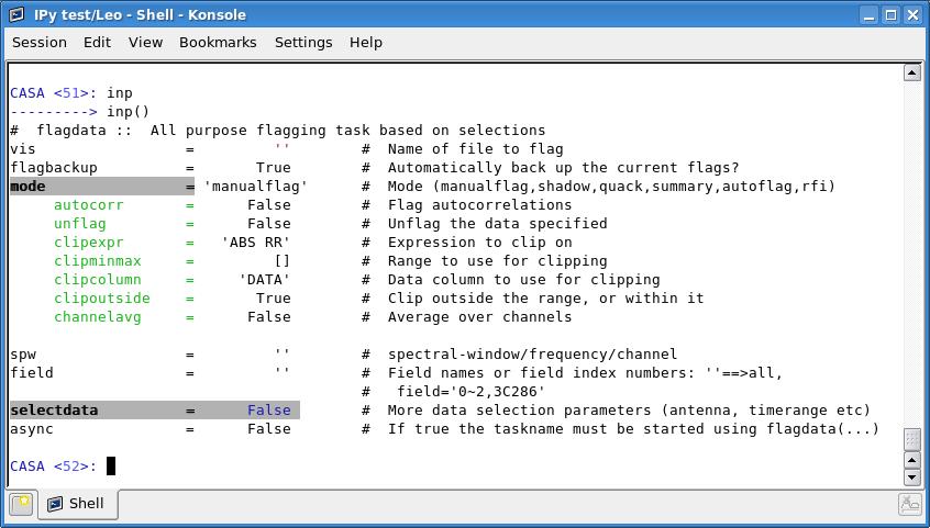
Oftentimes, the first few integrations of each scan are bad, and we'd like to flag them (IS QUACK STILL NECESSARY WITH WIDAR?). This is called 'quack' a la AIPS, and is implemented using flagdata. This is what the default flagdata parameters look like in our CASA window:
Tip: You'll notice that some parameters are colored differently than others. Standard parameters (familiar from AIPS) are simple black text (like vis above). Parameters which are shaded grey (like selectdata) are expandable, and once they have been expanded (like mode), green sub-parameters (like autocorr) will appear. Note that if you were to change mode from 'manualflag' to, say, 'quack', a different menu of green sub-parameters would appear.
To quack the first 10 seconds of each scan, set the flagdata parameters to:
#  flagdata ::  All purpose flagging task based on selections
vis                 = 'leotest.ms'      #  Name of file to flag
flagbackup          =       True        #  Automatically back up the current flags?
mode                =    'quack'        #  Mode (manualflag,shadow,quack,summary,autoflag,rfi)
     autocorr       =      False        #  Flag autocorrelations
     unflag         =      False        #  Unflag the data specified
     quackinterval  =         10        #  Quack n seconds from scan beginning/end
     quackmode      =      'beg'        #  Quack mode. 'beg' ==> beginning of scan. 'endb' ==> end of
                                        #   scan. 'end' ==> all but end of scan. 'tail' ==> all but
                                        #   beginning of scan
     quackincrement =      False        #  Flag incrementally in time?

spw                 =         ''        #  spectral-window/frequency/channel
field               =         ''        #  Field names or field index numbers: ''==>all,
                                        #   field='0~2,3C286'
selectdata          =      False        #  More data selection parameters (antenna, timerange etc)
async               =      False        #  If true the taskname must be started using flagdata(...)
Now is also the time to flag any obviously aberrant data in your calibrators. You might choose to flag with viewer, which displays a raster image of your uv data and is similar to SPFLG and TVFLG in AIPS (click here for an introduction to viewer). Alternatively, you can flag using a 2-dimensional interactive plot with plotms (click here for an introduction to plotms). The plotting capabilities can be likened to UVPLT in AIPS, and data points can be flagged (like WIPER in AIPS).
Calibration
Set the Flux Scale
Use the task setjy to find the flux density of the flux calibrator (as in AIPS). In this case, the flux calibrator is 1331+305.
#  setjy :: Fills the model column with the visibility of a calibrator
vis                 = 'leotest.ms'      #  Name of input visibility file
field               = '1331+305'        #  One Field name
spw                 =         ''        #  Spectral window identifier (list)
modimage            = '/home/casa/data/nrao/VLA/CalModels/3C286_L.im' #  File location for field model
fluxdensity         =         -1        #  Specified flux density [I,Q,U,V]; -1 will lookup values
standard            = 'Perley-Taylor 99' #  Flux density standard
async               =      False        #  If true the taskname must be started using setjy(...)
In most cases, you should be wary that the flux calibrator could be resolved, and you should use a model (set by the modimage parameter above). CASA comes pre-packed with model images, but finding them might be a bit tricky. Here are some probable paths (see the CASA Cookbook for more detail):
- Red Hat Linux RPMs (RHE4, Fedora 6): /usr/lib/casapy/data/nrao/VLA/CalModels
- MAC OSX .dmg: /opt/casa/data/nrao/VLA/CalModels
- NRAO-AOC stable: /home/casa/data/nrao/VLA/CalModels
You should also note that setjy expects your flux calibrator to be named in certain conventions (See Table 4.1 of the CASA Cookbook for acceptable names). If your observations don't follow these conventions, you'll probably have to change the flux calibrator's field name.
Setjy should output something that looks like this:
2010-02-11 23:57:53 INFO setjy	##########################################
2010-02-11 23:57:53 INFO setjy	##### Begin Task: setjy              #####
2010-02-11 23:57:53 INFO  	setjy::::casa
2010-02-11 23:57:53 INFO setjy	    1331+305  spwid=  0  [I=14.75, Q=0, U=0, V=0] Jy, (Perley-Taylor 99)
2010-02-11 23:57:54 INFO setjy	Using model image /home/casa/data/nrao/VLA/CalModels/3C286_L.im
2010-02-11 23:57:54 INFO setjy	The model image's reference pixel is 0.000254726 arcsec from 1331+305's phase center.
2010-02-11 23:57:54 INFO setjy	Scaling model image to I=14.7461 Jy for visibility prediction.
2010-02-11 23:57:54 INFO setjy	Selecting data
2010-02-11 23:57:54 INFO setjy	Selected 4818 out of 70290 visibilities.
2010-02-11 23:57:54 INFO setjy	Fourier transforming: replacing MODEL_DATA column
2010-02-11 23:57:54 INFO setjy	Performing interferometric gridding with convolution function SF
2010-02-11 23:57:55 INFO  	setjy::::casa
2010-02-11 23:57:55 INFO setjy	##### End Task: setjy                #####
2010-02-11 23:57:55 INFO setjy	##########################################
Note that it has determined a flux of 14.76 Jy for 1331+305. One of the most common signals that something has gone wrong is if setjy claims I=1 Jy.
Calibrate the Bandpasses
Let's use the flux calibrator to calibrate the bandpasses with the task bandpass (similar to BPASS in AIPS). 1331+305 now has a model image associated with it, so no preliminary gain calibration is needed (is this true??), and we can jump right in:
#  bandpass :: Calculates a bandpass calibration solution
vis                 = 'leotest.ms'      #  Nome of input visibility file
caltable            = 'leotest_1.bcal'  #  Name of output gain calibration table
field               = '1331+305'        #  Select field using field id(s) or field name(s)
spw                 =         ''        #  Select spectral window/channels
selectdata          =      False        #  Other data selection parameters
solint              =      'inf'        #  Solution interval
combine             =     'scan'        #  Data axes which to combine for solve (scan, spw, and/or field)
refant              =     'ea25'        #  Reference antenna name
minblperant         =          4        #  Minimum baselines _per antenna_ required for solve
solnorm             =       True        #  Normalize average solution amplitudes to 1.0 (G, T only)
bandtype            =        'B'        #  Type of bandpass solution (B or BPOLY)
     fillgaps       =          0        #  Fill flagged solution channels by interpolation

append              =      False        #  Append solutions to the (existing) table
gaintable           =       ['']        #  Gain calibration table(s) to apply on the fly
gainfield           =       ['']        #  Select a subset of calibrators from gaintable(s)
interp              =       ['']        #  Interpolation mode (in time) to use for each gaintable
spwmap              =         []        #  Spectral windows combinations to form for gaintables(s)
gaincurve           =      False        #  Apply internal VLA antenna gain curve correction
opacity             =        0.0        #  Opacity correction to apply (nepers)
parang              =      False        #  Apply parallactic angle correction
async               =      False        #  If true the taskname must be started using bandpass(...)
Important parameters to consider are:
- caltable: find an intuitive naming convention for your calibration tables. These calibration tables will be outputted as directories in your present working directory.
- field: the name of your bandpass calibrator
- refant: the reference antenna name
- solnorm: do you want your bandpass solutions to be normalized? I'm inclined to say Yes, I do. One case I've come across where solnorm=True was very important was where I had two different bandpass calibrator sources with quite different flux densities---one at the beginning of my observations and one at the end.
Now, run bandpass. You should get some helpful output in your CASA logger, and if you type 'ls' on the CASA command line, you should see a directory named for your caltable.
Tip: If, for some reason, you'd like to delete this caltable, the neatest way to do it is: rmtables('leotest_1.bcal') If you get an error when running rmtables, it is likely because CASA is still accessing the table. If you really want to delete the table, you'll have to quit out of CASA and then restart it.
We can also plot up our bandpass solutions with plotcal (which, in this case, can be likened to POSSM in AIPS with APARM(8)=2). Plotcal parameters that look like this:
#  plotcal :: An all-purpose plotter for calibration results
caltable            = 'leotest_1.bcal'  #  Name of input calibration table
xaxis               =         ''        #  Value to plot along x axis (time,chan,freq...see pdoc)
yaxis               =         ''        #  Value to plot along y axis (amp,phase,real,imag,snr,antenna)
poln                =         ''        #  Antenna polarization to plot (RL,R,L,XY,X,Y,/)
field               =         ''        #  field names or index of calibrators: ''==>all
antenna             =         ''        #  antenna/baselines: ''==>all, antenna = '3,VA04'
spw                 =         ''        #  spectral window:channels: ''==>all, spw='1:5~57'
timerange           =         ''        #  time range: ''==>all
subplot             =        111        #  Panel number on display screen (yxn)
overplot            =      False        #  Overplot solutions on existing display
clearpanel          =     'Auto'        #  Specify if old plots are cleared or not (ignore)
iteration           =  'antenna'        #  Iterate plots on antenna,time,spw,field
plotrange           =         []        #  plot axes ranges: [xmin,xmax,ymin,ymax]
showflags           =      False        #  If true, show flagged solutions
plotsymbol          =        'o'        #  pylab plot symbol
plotcolor           =     'blue'        #  initial plotting color
markersize          =        5.0        #  Size of plotted marks
fontsize            =       10.0        #  Font size for labels
showgui             =       True        #  Show plot on gui
figfile             =         ''        #  ''= no plot hardcopy, otherwise supply name
async               =      False        #  If true the taskname must be started using plotcal(...)
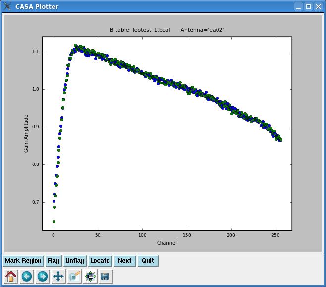
will plot the bandpass solutions (amplitude vs. channel) for each antenna individually. Note that if we had left iteration as its default:
iteration = '' # Iterate plots on antenna,time,spw,field
bandpasses for all antennae would be overplotted in the same window. By setting iteration= 'antenna', plotcal will plot bandpasses for each antenna separately. The plot can be advanced to the next antenna by clicking the ![]() button.
button.
If you want to plot the bandpass phase solutions, simply set yaxis= 'phase'. If you only want to plot one polarization, set the poln parameter. It is also possible to place multiple plots in one window using the subplot parameter; see the CASA Cookbook for more details.
Calibrate the Gains
Now it's time for amplitude and phase calibration with gaincal (analogous to CALIB in AIPS). If you are going to use the same uvrange for all calibrator sources, then you can run gaincal simultaneously on them all. Check with the calibrator manual to see the acceptable uvrange for each of your calibrators (if you have assigned a source model to your flux calibrator with setjy, then for that source you can ignore the suggested uvrange in the calibrator manual and use the full range). Here our phase calibrator (J1042+1203) has a suggested uvrange of 0--5 kilolambda, so we are going to run gaincal separately for the flux calibrator and the phase calibrator.
#  gaincal :: Determine temporal gains from calibrator observations
vis                 = 'leotest.ms'      #  Nome of input visibility file
caltable            = 'leotest_1.gcal'  #  Name of output gain calibration table
field               = '1331+305'        #  Select field using field id(s) or field name(s)
spw                 = '*:25~250'        #  Select spectral window/channels
selectdata          =      False        #  Other data selection parameters
solint              =      'inf'        #  Solution interval: egs. 'inf', '60s' (see help)
combine             =         ''        #  Data axes which to combine for solve (scan, spw, and/or field)
preavg              =       -1.0        #  Pre-averaging interval (sec) (rarely needed)
refant              =     'ea25'        #  Reference antenna name.  ' '= '0'
minblperant         =          4        #  Minimum baselines _per antenna_ required for solve
minsnr              =        0.0        #  Reject solutions below this SNR
solnorm             =      False        #  Normalize average solution amplitudes to 1.0 (G, T only)
gaintype            =        'G'        #  Type of gain solution (G, T, or GSPLINE)
calmode             =       'ap'        #  Type of solution" ('ap', 'p', 'a')
append              =      False        #  Append solutions to the (existing) table
gaintable           = 'leotest_1.bcal'  #  Gain calibration table(s) to apply on the fly
gainfield           =       ['']        #  Select a subset of calibrators from gaintable(s)
interp              =       ['']        #  Temporal interpolation for each gaintable (=linear)
spwmap              =         []        #  Spectral windows combinations to form for gaintables(s)
gaincurve           =      False        #  Apply internal VLA antenna gain curve correction
opacity             =        0.0        #  Opacity correction to apply on the fly (nepers)
parang              =      False        #  Apply parallactic angle correction on the fly
async               =      False        #  If true the taskname must be started using gaincal(...)
The above parameters calibrate the amplitudes and phases (calmode= 'ap') for the flux calibrator (field= '1331+305') and outputs the gain calibration to a table called 'leotest_1.gcal'. We only use channels 25--250 to calibrate (spw= '*:25~250'), chosen by visual inspection of the bandpass solutions with plotcal. The combination of parameters solint= 'inf' and combine= ' ' tell gaincal to time-integrate across an entire calibrator scan in finding a solution. In order for flux bootstrapping to work properly in the next calibration step, we want to refrain from normalizing the solutions (solnorm= False). Don't forget to set the reference antenna (refant= 'ea25') and apply the bandpass calibration (gaintable= 'leotest_1.bcal').
Next, we will calibrate the phase calibrator (field= 'J1042+1203') and set a limited uvrange (uvrange= '0~5klambda'):
#  gaincal :: Determine temporal gains from calibrator observations
vis                 = 'leotest.ms'      #  Nome of input visibility file
caltable            = 'leotest_1.gcal'  #  Name of output gain calibration table
field               = 'J1042+1203'      #  Select field using field id(s) or field name(s)
spw                 = '*:25~250'        #  Select spectral window/channels
selectdata          =       True        #  Other data selection parameters
     timerange      =         ''        #  Select data based on time range
     uvrange        = '0~5klambda'      #  Select data within uvrange (default units meters)
     antenna        =         ''        #  Select data based on antenna/baseline
     scan           =         ''        #  Scan number range
     msselect       =         ''        #  Optional complex data selection (ignore for now)
solint              =      'inf'        #  Solution interval: egs. 'inf', '60s' (see help)
combine             =         ''        #  Data axes which to combine for solve (scan, spw, and/or field)
preavg              =       -1.0        #  Pre-averaging interval (sec) (rarely needed)
refant              =     'ea25'        #  Reference antenna name.  ' '= '0'
minblperant         =          4        #  Minimum baselines _per antenna_ required for solve
minsnr              =        0.0        #  Reject solutions below this SNR
solnorm             =      False        #  Normalize average solution amplitudes to 1.0 (G, T only)
gaintype            =        'G'        #  Type of gain solution (G, T, or GSPLINE)
calmode             =       'ap'        #  Type of solution" ('ap', 'p', 'a')
append              =       True        #  Append solutions to the (existing) table
gaintable           = 'leotest_1.bcal'  #  Gain calibration table(s) to apply on the fly
gainfield           =       ['']        #  Select a subset of calibrators from gaintable(s)
interp              = ['linear']        #  Temporal interpolation for each gaintable (=linear)
spwmap              =         []        #  Spectral windows combinations to form for gaintables(s)
gaincurve           =      False        #  Apply internal VLA antenna gain curve correction
opacity             =        0.0        #  Opacity correction to apply on the fly (nepers)
parang              =      False        #  Apply parallactic angle correction on the fly
async               =      False        #  If true the taskname must be started using gaincal(...)
Note that we appended this calibration (append= True) to the original calibration table (caltable= 'leotest_1.gcal').
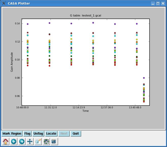
We'll check our gain solutions with plotcal. If we give it a gain table, the default plot will be amplitude vs. time (in this manifestation, plotcal can be likened to SNPLT in AIPS). The plot for our calibration can be seen to the right, with all antennae overplotted in different colors. We'll also want to check phase vs. time.
Apply the Flux Scale
Next, we'll bootstrap the flux scale that was found by running setjy onto our phase calibrator with the CASA task fluxscale (synonymous with GETJY in AIPS).
#  fluxscale :: Bootstrap the flux density scale from standard calibrators
vis                 = 'leotest.ms'      #  Name of input visibility file (MS)
caltable            = 'leotest_1.gcal'  #  Name of input calibration table
fluxtable           = 'leotest_1.fluxscale' #  Name of output, flux-scaled calibration table
reference           = '1331+305'        #  Reference field name(s) (transfer flux scale FROM)
transfer            = 'J1042+1203'      #  Transfer field name(s) (transfer flux scale TO), '' -> all
append              =       True        #  Append solutions?
refspwmap           =       [-1]        #  Scale across spectral window boundaries.  See help fluxscale
async               =      False        #  If true the taskname must be started using fluxscale(...)
We get output like this:
2010-02-14 21:35:04 INFO fluxscale	##########################################
2010-02-14 21:35:04 INFO fluxscale	##### Begin Task: fluxscale          #####
2010-02-14 21:35:04 INFO  	fluxscale::::casa
2010-02-14 21:35:04 INFO fluxscale	Opening MS: leotest.ms for calibration.
2010-02-14 21:35:04 INFO fluxscale	Initializing nominal selection to the whole MS.
2010-02-14 21:35:04 INFO fluxscale	Beginning fluxscale--(MSSelection version)-------
2010-02-14 21:35:04 INFO fluxscale	 Found reference field(s): 1331+305
2010-02-14 21:35:04 INFO fluxscale	 Found transfer field(s):  J1042+1203
2010-02-14 21:35:04 INFO fluxscale	 Flux density for J1042+1203 in SpW=0 is: 3.09102 +/- 0.0129722 (SNR = 238.28, nAnt= 12)
2010-02-14 21:35:04 INFO fluxscale	Appending result to leotest_1.fluxscale
2010-02-14 21:35:04 INFO fluxscale	Appending solutions to table: leotest_1.fluxscale
2010-02-14 21:35:04 INFO  	fluxscale::::casa
2010-02-14 21:35:04 INFO fluxscale	##### End Task: fluxscale            #####
which tells us that our phase calibrator has a flux density of 3.1 Jy. Here, it is good to be on guard for flux densities which are suspiciously close to 1 Jy or errors in the derived flux density which are very large. Note that, unlike in AIPS, fluxscale writes a new calibration table, and this is what we will want to apply to our data.
Apply the Calibration
Now, we're happy with our calibration and ready to apply it to the data with applycal. This task might be compared with CLCAL in AIPS, except that instead of writing a new calibration (CL) table, applycal will write a new calibrated column of data in your '.ms' file. After we run applycal, we will still be able to access the raw data (called 'data' by many tasks), but there will also be calibrated data (called 'corrected' by many tasks).
#  applycal :: Apply calibrations solutions(s) to data
vis                 = 'leotest.ms'      #  Nome of input visibility file
field               =         ''        #  Select field using field id(s) or field name(s)
spw                 =         ''        #  Select spectral window/channels
selectdata          =      False        #  Other data selection parameters
gaintable           = ['leotest_1.bcal', 'leotest_1.fluxscale'] #  Gain calibration table(s) to apply on the fly
gainfield           =       ['']        #  Select a subset of calibrators from gaintable(s)
interp              =   'linear'        #  Temporal Interpolation type.  default=linear
spwmap              =         []        #  Spectral windows combinations to form for gaintables(s)
gaincurve           =      False        #  Apply internal VLA antenna gain curve correction
opacity             =        0.0        #  Opacity correction to apply (nepers)
parang              =      False        #  Apply parallactic angle correction
calwt               =       True        #  Calibrate data weights from all relevant calibrations
async               =      False        #  If true the taskname must be started using applycal(...)
The above settings for applycal will only calibrate all sources, linearly interpolating between gaincal solutions. It will apply the flux, gain, and bandpass calibration (gaintable= ['leotest_1.bcal', 'leotest_1.fluxscale']).
Inspect the Calibrated Data
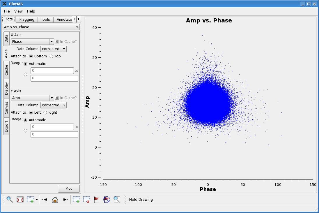
A good way to check our calibration is to plot up amplitudes and phases for our calibrated calibrators. By default plotms plots up the raw data column of a '.ms' file. If, at this point, we were to leave the plotms parameters as their defaults and plot up amplitude vs. phase for 1331+305, we'd see a plot that looks like this:
To plot the calibrated data, go to the plotms window and click on the Axes tab. You will see drop-down menus called Data Column. Select 'corrected', and the plot should now look like this:
A nice ball, just as we'd expect from calibrated data. Also note that the amplitudes are centered around ~15 Jy, consistent with what was found from setjy.
You can also easily switch between raw and calibrated data in viewer by selecting a Visibility Type, which can be found in MS and Visibility Selection section of the Data Display Options window. There will be a choice of 'observed' or 'corrected' visibilities. You can even display the 'model' and 'residual' visibilities!
After calibration, new bad data will often pop up [IS THIS STILL TRUE WITH WIDAR??]. If there are a lot of bad data or the bad points are severely aberrant, you might want to take this opportunity to flag them and then recalibrate the data. In this case, it is probably good form to delete the corrected data column with clearcal (but note that this task can be quite slow, and this step may be unnecessary as gaincal and bandpass will, regardless, use the raw data, and applycal will overwrite the old 'corrected' data if it is run again). Then start again from the bandpass step above (making sure to give calibration tables different names).
Split Off the Science Targets
Finally, we'll want to split off our calibrated science targets from the multi-source measurement set, so that we can image them! Use split, just as you would in AIPS.
#  split :: Create a visibility subset from an existing visibility set
vis                 = 'leotest.ms'      #  Name of input measurement set
outputvis           = 'leo1_split.ms'   #  Name of output measurement set
datacolumn          = 'corrected'       #  Which data column(s) to split out
field               =    'Leo-1'        #  Select field using field id(s) or field name(s)
spw                 = '*:25~250'        #  Select spectral window/channels
width               =        '1'        #  Number of channels to average to form one output channel
antenna             =         ''        #  Select data based on antenna/baseline
timebin             =        '0'        #  Value for timeaveraging
timerange           =         ''        #  Select data based on time range
scan                =         ''        #  select data based on scan numbers
array               =         ''        #  Select (sub)array by array ID number(s)
uvrange             =         ''        #  select data based on uv distance range
async               =      False        #  If true the taskname must be started using split(...)
The above will split off the calibrated data (datacolumn= 'corrected') for first Leo field (field= 'Leo-1'). We're only including the "good" channels 25--250 in the new single-source data set. We'll also want to repeat the above for the second Leo pointing, 'Leo-2'.
Now we are ready to flag these science targets and image them! Continue on to this imaging tutorial for the next installment....
--Laura Chomiuk 23:35, 14 February 2010 (UTC)
