Imaging an EVLA OSRO HI data set
Overview
This tutorial explains how to image an HI dataset acquired with the WIDAR0 correlator. It assumes that you've already calibrated your data as described in the calibration tutorial, and that you now have a split dataset with a single source of interest in it. In this example, the source is called 'Leo-2'; see the calibration tutorial for more details on this data set.
Flag Your Split Data
You'll want to make sure that no new bad data has popped up in your science targets post-calibration. Load the split dataset into plotms and/or viewer and flag any bad data.
For a spectral line dataset like this one, you'll probably want to average in various ways to spot bad data. Averaging channels together can make bad baselines pop up!
Doppler Tracking
Presently, doppler tracking is not performed online by the EVLA, so we have to correct for any velocity shifts now, in post-processing, with cvel.
#  cvel :: regrid an MS to a new spectral window / channel structure or frame
vis                 =  'leo2.ms'        #  Name of input measurement set
outputvis           = 'leo2_cvel.ms'    #  Name of output measurement set
passall             =      False        #  Pass through (write to output MS) non-selected data with no change
field               =         ''        #  Select field using field id(s) or field name(s)
spw                 =        '0'        #  Select spectral window/channels
selectdata          =      False        #  Other data selection parameters
mode                =  'channel'        #   Regridding mode
     nchan          =         -1        #  Number of channels in output spw (-1=all)
     start          =          0        #  first input channel to use
     width          =          1        #  Number of input channels to average
     interpolation  =   'linear'        #  Spectral interpolation method

phasecenter         =         ''        #  Image phase center: position or field index
restfreq            = '1420405751.786Hz' #  rest frequency (see help)
outframe            =     'BARY'        #  Output frame (''=keep input frame)
veltype             =    'radio'        #  velocity definition
hanning             =      False        #  Turn on Hanning smoothing of spectral channels
async               =      False        #  If true the taskname must be started using cvel(...)
Cvel creates a new measurement set (outputvis= 'leo2_cvel.ms') for which, at each time, the spectrum has been shifted and channels regridded to keep the spectral line centered in the frame of your choice (here, we choose barycentric; outframe= 'BARY'). You'll also want to give cvel the rest frequency of your spectral line (restfreq= '1420405751.786Hz' for HI).
Continuum Subtraction
|
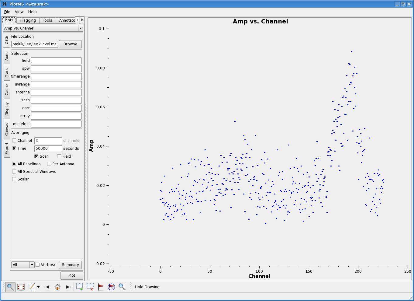
In preparation for subtracting the continuum, let us plot up the combined spectrum on our science field and identify some line-free channels. Open up a plotms GUI window and load the doppler-tracked measurement set containing your science target. You'll want to average over both time and baselines to get as much signal-to-noise as possible, hopefully revealing a nice 21 cm profile. In the Data tab of plotms, set the below averaging options:
(See Averaging data in plotms for more details on averaging options). You'll also want to click on the Axes tab in the plotms window, and change the axes settings to:
The figure to the right shows the resulting plot in plotms. There is clearly some line emission around channel 190, and possibly some faint emission around channel 88. Let's use channels 10--55 and 120--155 to fit the continuum. |
Next, use uvcontsub to subtract the continuum from your data set. Here are the parameters we used:
#  uvcontsub :: Continuum fitting and subtraction in the uv plane
vis                 =  'leo2_cvel.ms'        #  Name of input visibility file
field               =         ''        #  Select field using field id(s) or field name(s)
fitspw              = '0:10~55;120~155' #  Spectral window/channel selection for fitting the continuum
spw                 =        '0'        #  Spectral window selection for subtraction/export
solint              =      '60s'        #  Continuum fit timescale
fitorder            =          0        #  Polynomial order for the fit
fitmode             = 'subtract'        #  Use of continuum fit (subtract,replace,model)
splitdata           =       True        #  Split out continuum, continuum-subtracted data
async               =      False        #  If true the taskname must be started using uvcontsub(...)
Here, we are fitting the continuum to channels 10--55 and 120--155 of spectral window 0 (the only spectral window). See this description for more detail on selecting spectral windows and channels. We're averaging over one minute intervals (solint= '60s') before fitting the continuum; note that the default will fit each integration (so, every one second for un-averaged EVLA data). We're fitting a simple mean to the continuum (fitorder= 0), although higher-order fits are certainly possible.
Note that the form of the output from uvcontsub can be a bit confusing, and depends on your choice of the fitmode and splitdata parameters. If splitdata= True, two new measurement sets will be created: one with the fitted continuum data ('leo2_cvel.ms.cont') and one with the continuum-subtracted data ('leo2_cvel.ms.contsub'). Uvcontsub will also alter your 'corrected' and 'model' data columns---exactly how depends on your choice of fitmode. We have set fitmode= 'subtract', which means the fitted continuum values are placed in the 'model' column, and the continuum-subtracted data are placed in the 'corrected' column.
If you have previously applied a calibration to the measurement set that you now want to continuum-subtract (with applycal, so that the 'data' and 'corrected' columns are different), note that uvcontsub will overwrite the 'corrected' data column. In this case, it is best to first create a new calibrated measurement set using split (datacolumn= 'corrected'), and then run uvcontsub on that newly-split data set.
Make an Image Cube (Interactively)
|
It's finally time to make an image! Imaging in CASA should be done with clean, including mosaicing. Here, we discuss interactive imaging/deconvolution, but see the NGC 5921 tutorial for an example of non-interactive imaging. # clean :: Invert and deconvolve images with selected algorithm
vis = 'leo2_cvel.ms.contsub' # Name of input visibility file
imagename = 'leo2_cube' # Pre-name of output images
outlierfile = '' # Text file with image names, sizes, centers for outliers
field = '' # Field Name or id
spw = '' # Spectral windows e.g. '0~3', '' is all
selectdata = False # Other data selection parameters
mode = 'channel' # Spectral gridding type (mfs, channel, velocity, frequency)
nchan = -1 # Number of channels (planes) in output image; -1 = all
start = 0 # First channel to use (0=first channel specified in spw)
width = 1 # Number of input channels to average
interpolation = 'linear' # Spectral interpolation (nearest, linear, cubic)
outframe = '' # velocity frame of output image
gridmode = '' # Gridding kernel for FFT-based transforms, default='' None
niter = 10000 # Maximum number of iterations
gain = 0.1 # Loop gain for cleaning
threshold = '0.0mJy' # Flux level to stop cleaning, must include units: '1.0mJy'
psfmode = 'hogbom' # Method of PSF calculation to use during minor cycles
imagermode = 'csclean' # Options: 'csclean' or 'mosaic', '', uses psfmode
cyclefactor = 1.5 # change depth in between of csclean cycle
cyclespeedup = -1 # Cycle threshold doubles in this number of iteration
multiscale = [] # Deconvolution scales (pixels); [] = standard clean
interactive = True # Use interactive clean (with GUI viewer)
npercycle = 20 # Clean iterations before interactive prompt (can be changed)
chaniter = False # Clean each channel to completion (True), or all channels each cycle (False)
mask = '' # Cleanbox(es), mask image(s), and/or mask region(s)
imsize = [256, 256] # x and y image size in pixels. Single value: same for both
cell = ['12.0arcsec', '12.0arcsec'] # x & y cell size(s). Default unit arcsec.
phasecenter = '' # Image center: direction or field index
restfreq = '1420405751.786Hz' # Rest frequency to assign to image (see help)
stokes = 'I' # Stokes params to image (eg I,IV, QU,IQUV)
weighting = 'natural' # Weighting of uv (natural, uniform, briggs, ...)
uvtaper = False # Apply additional uv tapering of visibilities
modelimage = '' # Name of model image(s) to initialize cleaning
restoringbeam = [''] # Output Gaussian restoring beam for CLEAN image
pbcor = False # Output primary beam-corrected image
minpb = 0.2 # Minimum PB level to use
calready = True # True required for self-calibration
async = False # If true the taskname must be started using clean(...)
clean()
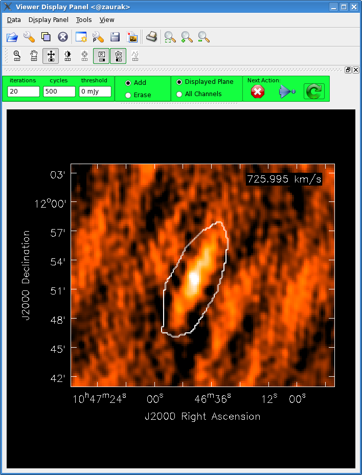
The viewer which pops up during interactive clean |
This will create an image cube called 'leo2_cube.image', along with some other relevant files (all with the prefix 'leo2_cube'). We are making a cube (mode= 'channel') which includes all channels in our measurement set (nchan= -1, start= 0). Each image plane will be 256x256 pixels (imsize) and each pixel is 12x12 arcseconds (cell). The images will be made with the natural weighting (weighting= 'natural').
The deconvolution will proceed interactively (interactive= True); each interactive deconvolution cycle will clean npercycle iterations for each channel with a clean box. It is recommended to start with this number small (npercycle= 20 or so) and then increase it interactively as the cleaning proceeds. If you're planning on continuing with interactive deconvolution until you are satisfied that all flux has been cleaned, simply set niter to a large value so it will not prematurely terminate clean. However, if you are planning on switching over to non-interactive deconvolution at some point (e.g., after you are confident in your clean boxes), you'll want to set niter and/or threshold thoughtfully. The first channel in the cube to undergo niter iterations of deconvolution will signal clean to end. Alternatively, threshold can be set, telling clean to clean down to a specified flux level. If threshold= '0.0mJy', clean will ignore threshold and only use niter; if both threshold and niter are set, clean will stop when it hits the first of these limits.
|
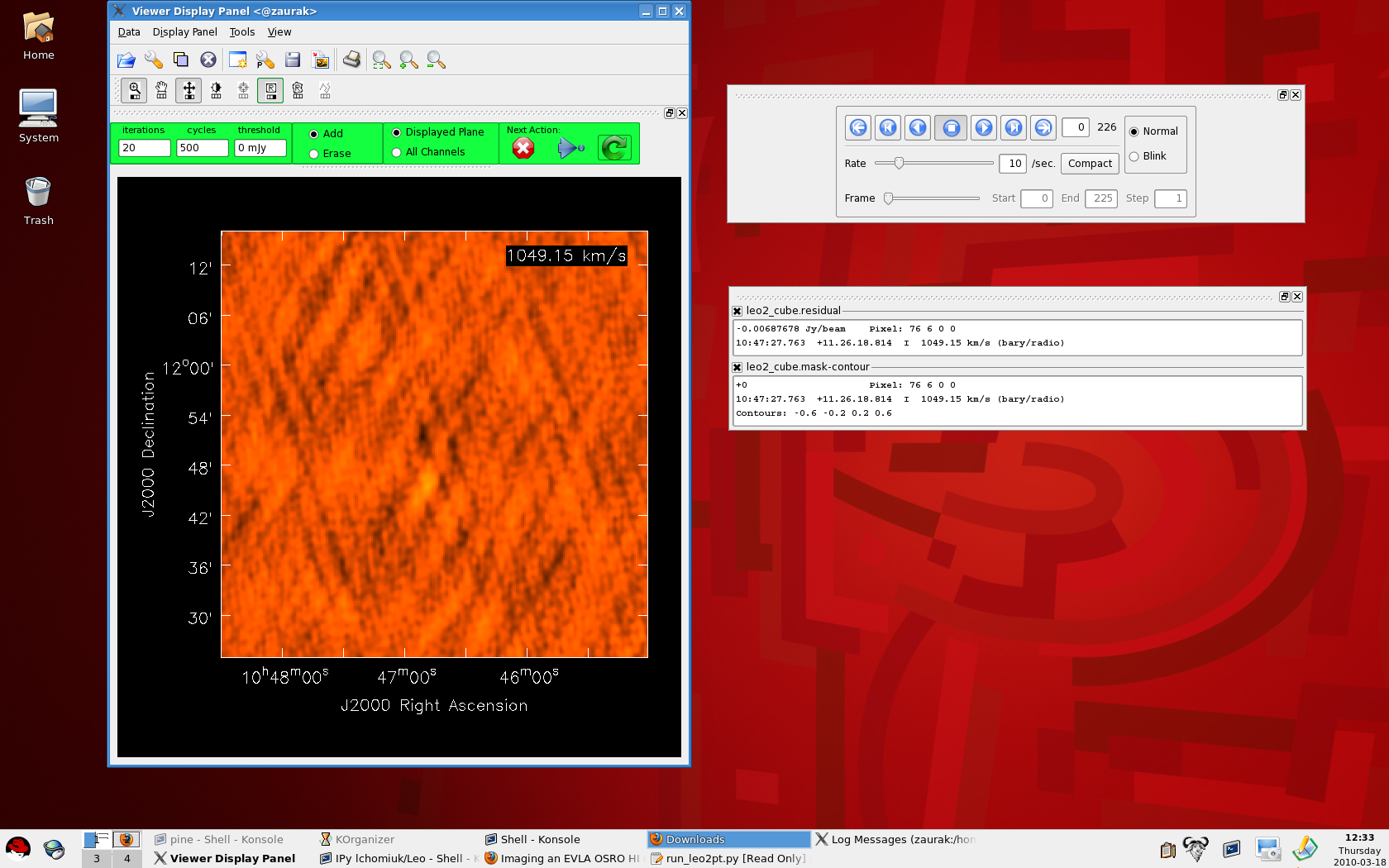
Wait while CASA processes your measurement set, producing output that looks like this on the command line: ---------> go(clean) Executing: clean() 0%....10....20....30....40....50....60....70....80....90....100% 0%....10....20....30....40....50....60....70....80....90....100% After the second '100%', a viewer window will pop up with your dirty image cube (like the figure above and to the right). You can make the image itself bigger in the viewer by clicking on the dashed line above the panel with the DVD-like control buttons and dragging it onto your desktop. Similarly, you can also drag the bottom-most panel which tracks your mouse and displays basic image information out of the viewer and on to the desktop (see the figure to the right). To view different channels, use the DVD-like control panel. The Drag panels out of the viewer and on to your desktop to enlarge the image |
|
After getting a good look at the image cube in viewer, it's time to start setting clean boxes. For this, we'll use the Clean will then clean npercycle iterations (here set to 20) from each channel with a clean box in it. When it has completed this, the viewer will become active again and you can place more clean boxes if necessary. You can also increase the number of clean iterations between interactive cycles by typing a larger number in the Iterations box in the viewer window. When ready, click the |
Reusing Clean Boxes
You've just spent a lot of time setting clean boxes on an image, but now you've realized that the last imaging run wasn't perfect, and you'd like to run clean again---without having to reset all those clean boxes. Luckily, the clean boxes were saved last time in a file called 'leo2_cube.mask'. Just rerun clean with mask= 'leo2_cube.mask', and it will use your clean boxes from that previous imaging run.
Warning: There is currently a bug in clean where, if you give it a mask file, you will not be able to add additional clean boxes; you are stuck with those in the mask file. This less-than-ideal situation will be fixed in a future release of CASA.
Primary Beam Correction
You'll probably want to perform a primary beam correction on any image you create (as AIPS users do with PBCOR). You can instruct clean to make this correction by setting pbcor= True, but it is more handy and flexible to make the primary beam correction after imaging with immath.
#  immath :: Perform math operations on images
imagename           = ['leo2_cube.image', 'leo2_cube.flux'] #  a list of input images
mode                = 'evalexpr'        #  mode for math operation (evalexpr, spix, pola, poli)
     expr           = 'IM0/IM1[IM1>0.023]' #  Mathematical expression using images
     varnames       =         ''        #  a list of variable names to use with the image files

outfile             = 'leo2_cube.pbcor' #  File where the output is saved
mask                =         []        #  Mask to be applied to the images
region              =         ''        #  File path which contains an Image Region
box                 =         ''        #  Select one or more box regions in the input images
chans               =         ''        #  Select the channel(spectral) range
stokes              =        'I'        #  Stokes params to image (I,IV,IQU,IQUV)
async               =      False        #  If true the taskname must be started using immath(...)
The 'leo2_cube.flux' image is one of the extra files created by clean, and is a model of the primary beam. Here, we are using immath to divide the science image cube ('leo2_cube.image') by the '.flux' image. By stating imagename= ['leo2_cube.image', 'leo2_cube.flux'], we are labeling 'leo2_cube.image' as IM0 and 'leo2_cube.flux' as IM1. In evalexpr mode, we can manipulate these two images in a variety of ways, but here we divide them (expr= 'IM0/IM1'). We also blank the pixels at the edges of the primary beam, where sensitivity is less that 2.3% of peak ('[IM1>0.023]'; the default cutoff in AIPS PBCOR). The new image cube with primary-beam correction is output as outfile.
Image Statistics
There are several ways to measure statistics on your image cube. The simplest is to just run imstat:
#  imstat :: Displays statistical information from an image or image region
imagename           = 'leo2_cube.image' #  Name of the input image
region              =         ''        #  Image Region or name. Use Viewer
box                 =         ''        #  Select one or more box regions
chans               =         ''        #  Select the channel(spectral) range
stokes              =        'I'        #  Stokes params to image (I,IV,IQU,IQUV)
async               =      False        #  If true the taskname must be started using imstat(...)
which will output something that looks like this:
2010-03-18 17:01:33 INFO imstat	##########################################
2010-03-18 17:01:33 INFO imstat	##### Begin Task: imstat             #####
2010-03-18 17:01:33 INFO  	imstat::::casa
2010-03-18 17:01:33 INFO imstat	Created Box at: [0, 0, 0, 0]  [511, 511, 0, 225]
2010-03-18 17:01:33 INFO imregion	Selected bounding box :
2010-03-18 17:01:33 INFO imregion	    [0, 0, 0, 0] to [511, 511, 0, 225]  (10:48:29.468, +11.25.00.788, I, 1.415571e+09Hz to 10:45:00.615, +12.16.06.822, I, 1.417329e+09Hz)
2010-03-18 17:01:33 INFO imregion	Regions ---
2010-03-18 17:01:33 INFO imregion	         -- bottom-left corner (pixel) [blc]:  [0, 0, 0, 0]
2010-03-18 17:01:33 INFO imregion	         -- top-right corner (pixel) [trc]:    [511, 511, 0, 225]
2010-03-18 17:01:33 INFO imregion	         -- bottom-left corner (world) [blcf]: 10:48:29.468, +11.25.00.788, I, 1.415571e+09Hz
2010-03-18 17:01:33 INFO imregion	         -- top-right corner (world) [trcf]:   10:45:00.615, +12.16.06.822, I, 1.417329e+09Hz
2010-03-18 17:01:44 INFO imregion	Values ---
2010-03-18 17:01:44 INFO imregion	         -- flux density [flux]:     -7.76782 Jy
2010-03-18 17:01:44 INFO imregion	         -- number of points [npts]:                5.92445e+07
2010-03-18 17:01:44 INFO imregion	         -- maximum value [max]:                    0.0852988 Jy/beam
2010-03-18 17:01:44 INFO imregion	         -- minimum value [min]:                    -0.0699967 Jy/beam
2010-03-18 17:01:44 INFO imregion	         -- position of max value (pixel) [maxpos]: [261, 269, 0, 192]
2010-03-18 17:01:44 INFO imregion	         -- position of min value (pixel) [minpos]: [0, 406, 0, 149]
2010-03-18 17:01:44 INFO imregion	         -- position of max value (world) [maxposf]: 10:46:42.956, +11.51.56.000, I, 1.417071e+09Hz
2010-03-18 17:01:44 INFO imregion	         -- position of min value (world) [maxposf]: 10:48:29.725, +12.05.36.802, I, 1.416735e+09Hz
2010-03-18 17:01:44 INFO imregion	         -- Sum of pixel values [sum]:               -496.171 Jy/beam
2010-03-18 17:01:44 INFO imregion	         -- Sum of squared pixel values [sumsq]:     5228.59 Jy/beam.Jy/beam
2010-03-18 17:01:44 INFO  	imregion::::
2010-03-18 17:01:44 INFO imregion	Statistics ---
2010-03-18 17:01:44 INFO imregion	        -- Mean of the pixel values [mean]:         -8.37496e-06 Jy/beam
2010-03-18 17:01:44 INFO imregion	        -- Variance of the pixel values :           8.82542e-05 Jy/beam
2010-03-18 17:01:44 INFO imregion	        -- Standard deviation of the Mean [sigma]:  0.00939437 Jy/beam
2010-03-18 17:01:44 INFO imregion	        -- Root mean square [rms]:                  0.00939438 Jy/beam
2010-03-18 17:01:44 INFO imregion	        -- Median of the pixel values [median]:     -2.59749e-05 Jy/beam
2010-03-18 17:01:44 INFO imregion	        -- Median of the deviations [medabsdevmed]: 0.00621969 Jy/beam
2010-03-18 17:01:44 INFO imregion	        -- Quartile [quartile]:                     0.0124394 Jy/beam
2010-03-18 17:01:44 INFO  	imstat::::casa
2010-03-18 17:01:44 INFO imstat	##### End Task: imstat               #####
2010-03-18 17:01:44 INFO imstat	##########################################
Note that in this case, imstat was run on the entire image and all channels. To find statistics over a subset of pixels, set the parameters box (with the syntax 'xmin, ymin, xmax, ymax', reminiscent of the BLC/TRC box definition in AIPS; e.g., box= '10,10,50,50'). To find statistics over a subset of channels, set the chans parameter (this will include all spectral windows; proper syntax is chans= '128' or chans= '3~20'). You can also define regions in viewer and then input them to imstat; more details on this soon.
Another way to get image statistics is to start up viewer, load your image as a Raster Image, and make a region using the ![]() and
and ![]() buttons (much as you did above in clean). This time, when you double-click in the green region, statistics within the region will be measured and displayed on the CASA command line.
buttons (much as you did above in clean). This time, when you double-click in the green region, statistics within the region will be measured and displayed on the CASA command line.
Warning: Currently, these are statistics integrated through the entire data cube. Viewer in future releases of CASA will provide single-channel statistics.
Other Analysis
Check out the NGC 5921 tutorial for a discussion of image moments and integrated spectra.
Last checked on CASA Version 3.0.1 (r10803).
--Laura Chomiuk 20:49, 18 March 2010 (UTC)


