Simulating Observations in CASA draft: Difference between revisions
| Line 25: | Line 25: | ||
A detailed overview of <b>how to simulate data in CASA</b> is given in the "Simulation" pages of the {{casadocs_6.6.1}} documentation. The following tutorials provide additional examples: | A detailed overview of <b>how to simulate data in CASA</b> is given in the "Simulation" pages of the {{casadocs_6.6.1}} documentation. The following tutorials provide additional examples: | ||
{| style="width: 100%; valign: top | {| style="width: 100%; valign: top; border:1px solid; text-align: center; cellpadding=10" | ||
! [[Simulating ngVLA Data]] (CASA 5.4.1) | ! [[Simulating ngVLA Data]] (CASA 5.4.1) | ||
| rowspan=2; stype="border-bottom:1px solid black;" | [[File:ngVLA_pic.png| | | rowspan=2; stype="border-bottom:1px solid black;" | [[File:ngVLA_pic.png|200px]] | ||
|- | |- | ||
| style="border-bottom:1px solid black;" | This tutorial shows how to create simulated data for the next generation Very Large Array (ngVLA) either by using simobserve or the sm toolkit. Additionally, it shows how to estimate the scaling parameter for adding thermal noise using the sm.setnoise function and the simplenoise parameter. | | style="border-bottom:1px solid black;" | This tutorial shows how to create simulated data for the next generation Very Large Array (ngVLA) either by using simobserve or the sm toolkit. Additionally, it shows how to estimate the scaling parameter for adding thermal noise using the sm.setnoise function and the simplenoise parameter. | ||
| Line 34: | Line 34: | ||
! [[Simalma CASA 6.5.4]] | ! [[Simalma CASA 6.5.4]] | ||
| rowspan=3; style="border-bottom:1px solid black;" | [[File:M51c.ALMA 0.5arcsec.skymodel.png| | | rowspan=3; style="border-bottom:1px solid black;" | [[File:M51c.ALMA 0.5arcsec.skymodel.png|250px]] | ||
|- | |- | ||
|Version History: [6.4][6.2][5.6][5.4][4.3] | |Version History: [6.4][6.2][5.6][5.4][4.3] | ||
| Line 42: | Line 42: | ||
! [[ACA Simulation CASA 6.5.4]] | ! [[ACA Simulation CASA 6.5.4]] | ||
| rowspan=2; style="border-bottom:1px solid black;" | [[File:M51c.ALMA 0.5arcsec.skymodel.png| | | rowspan=2; style="border-bottom:1px solid black;" | [[File:M51c.ALMA 0.5arcsec.skymodel.png|250px]] | ||
|- | |- | ||
| style="border-bottom:1px solid black;" | A tutorial for simulating ALMA observations that use multiple configurations or use the 12-meter array in combination with the ALMA Compact Array. This tutorial demonstrates combining data from each ALMA component "by hand". This guide is of particular interest to those wishing to explore using the 12-m array in combination with the ACA, and those interested in combining data from multiple 12-m array configurations. | | style="border-bottom:1px solid black;" | A tutorial for simulating ALMA observations that use multiple configurations or use the 12-meter array in combination with the ALMA Compact Array. This tutorial demonstrates combining data from each ALMA component "by hand". This guide is of particular interest to those wishing to explore using the 12-m array in combination with the ACA, and those interested in combining data from multiple 12-m array configurations. | ||
| Line 48: | Line 48: | ||
! [[Simulation Guide Component Lists (CASA 6.5.3)]] | ! [[Simulation Guide Component Lists (CASA 6.5.3)]] | ||
| rowspan=2; style="border-bottom:1px solid black;" | [[File:Analyze_fits_list.jpg| | | rowspan=2; style="border-bottom:1px solid black;" | [[File:Analyze_fits_list.jpg|200px]] | ||
|- | |- | ||
| style="border-bottom:1px solid black;" | Tutorial for simulating data based on multiple sources (using both a FITS image and a component list). If you are interested in simulating from a list of simple sources (point, Gaussian, disk), rather than or in addition to a sky model image, then read the considerations here. | | style="border-bottom:1px solid black;" | Tutorial for simulating data based on multiple sources (using both a FITS image and a component list). If you are interested in simulating from a list of simple sources (point, Gaussian, disk), rather than or in addition to a sky model image, then read the considerations here. | ||
| Line 54: | Line 54: | ||
! [[Protoplanetary Disk Simulation (CASA 5.4)]] | ! [[Protoplanetary Disk Simulation (CASA 5.4)]] | ||
| rowspan=2; stype="border-bottom:1px solid black;" | [[File:Psimthumb.png| | | rowspan=2; stype="border-bottom:1px solid black;" | [[File:Psimthumb.png|200px]] | ||
|- | |- | ||
| style="border-bottom:1px solid black;" | A sky model with a lightly annotated script that simulates a protoplanetary disk. Uses a theoretical model of dust continuum from Sebastian Wolff, scaled to the distance of a nearby star. This is another fairly generic simulation - if you're short on time, you probably don't need to go through this one and the New Users guide, but it can be useful to go through multiple examples. | | style="border-bottom:1px solid black;" | A sky model with a lightly annotated script that simulates a protoplanetary disk. Uses a theoretical model of dust continuum from Sebastian Wolff, scaled to the distance of a nearby star. This is another fairly generic simulation - if you're short on time, you probably don't need to go through this one and the New Users guide, but it can be useful to go through multiple examples. | ||
| Line 60: | Line 60: | ||
! [[Protoplanetary Disk Simulation - VLA]] (CASA 5.5) | ! [[Protoplanetary Disk Simulation - VLA]] (CASA 5.5) | ||
| rowspan=2; stype="border-bottom:1px solid black;" | [[File:VLAsim-psim4mfstclean.png| | | rowspan=2; stype="border-bottom:1px solid black;" | [[File:VLAsim-psim4mfstclean.png|200px]] | ||
|- | |- | ||
| style="border-bottom:1px solid black;" | This tutorial explains the steps for simulating VLA observations using the same protoplanetary disk sky model that was used for the analogous ALMA tutorial. Observational and analysis parameters are changed step by step and the results are compared to the VLA exposure calculator. | | style="border-bottom:1px solid black;" | This tutorial explains the steps for simulating VLA observations using the same protoplanetary disk sky model that was used for the analogous ALMA tutorial. Observational and analysis parameters are changed step by step and the results are compared to the VLA exposure calculator. | ||
| Line 72: | Line 72: | ||
|} | |} | ||
== Archived Simulation Guides == | == Archived Simulation Guides == | ||
| Line 78: | Line 77: | ||
<table> | <table> | ||
== Version History == | == Version History == | ||
Revision as of 23:15, 18 October 2024
Introduction
This page contains tutorials on how to simulate data in CASA. The two main CASA tasks that are used for this are simobserve and simanalyze. CASA includes configuration files for a large number of interferometers (ALMA, VLA, VLBA, ATCA, CARMA, SMA, PdBI and WSRT).
For ALMA, the Guide to Simulating ALMA Data gives an introduction to ALMA simulations, and discusses their relevance to ALMA observing proposals. The task simalma is available to simplify the process of simulating data that combines the 12-m Main Array and the ACA.
If you are a new user of CASA, take a look at CASA Docs (the official CASA Documentation).
If you are new to CASAguides, start with How To Use A CASAGuide.
General introduction to CASA simulations
Simulating interferometric observations in CASA proceeds in the following steps:
- Make a model image. The model image is a representation of the sky brightness distribution that you would like to simulate observing, stored initially as a FITS file. There are several paths to making the FITS file, discussed below.
- Generate uv data with the simobserve task.
- Image the simulated observation with the simanalyze task.
This page on "Introduction to CASA simulations" provides a detailed introduction on how to simulate interferometric data in CASA.
Tutorials
A detailed overview of how to simulate data in CASA is given in the "Simulation" pages of the CASA Docs documentation. The following tutorials provide additional examples:
| Simulating ngVLA Data (CASA 5.4.1) | 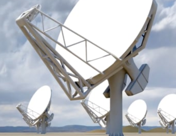
|
|---|---|
| This tutorial shows how to create simulated data for the next generation Very Large Array (ngVLA) either by using simobserve or the sm toolkit. Additionally, it shows how to estimate the scaling parameter for adding thermal noise using the sm.setnoise function and the simplenoise parameter. | |
| Simalma CASA 6.5.4 | 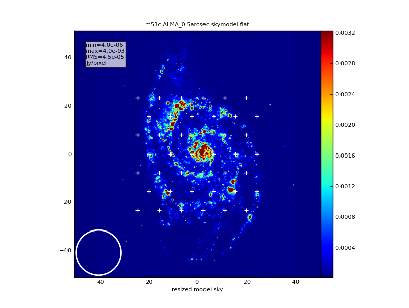
|
| Version History: [6.4][6.2][5.6][5.4][4.3] | |
| This tutorial demonstrates how to use simalma, a task that simplifies simulations that include the main 12-m array plus the ACA. Like the previous guide, this one is of particular interest to those wishing to explore multi-component ALMA observations. | |
| ACA Simulation CASA 6.5.4 | 
|
| A tutorial for simulating ALMA observations that use multiple configurations or use the 12-meter array in combination with the ALMA Compact Array. This tutorial demonstrates combining data from each ALMA component "by hand". This guide is of particular interest to those wishing to explore using the 12-m array in combination with the ACA, and those interested in combining data from multiple 12-m array configurations. | |
| Simulation Guide Component Lists (CASA 6.5.3) | 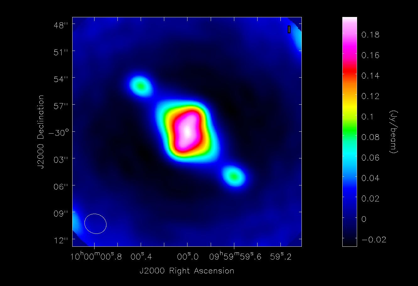
|
| Tutorial for simulating data based on multiple sources (using both a FITS image and a component list). If you are interested in simulating from a list of simple sources (point, Gaussian, disk), rather than or in addition to a sky model image, then read the considerations here. | |
| Protoplanetary Disk Simulation (CASA 5.4) | 
|
| A sky model with a lightly annotated script that simulates a protoplanetary disk. Uses a theoretical model of dust continuum from Sebastian Wolff, scaled to the distance of a nearby star. This is another fairly generic simulation - if you're short on time, you probably don't need to go through this one and the New Users guide, but it can be useful to go through multiple examples. | |
| Protoplanetary Disk Simulation - VLA (CASA 5.5) | 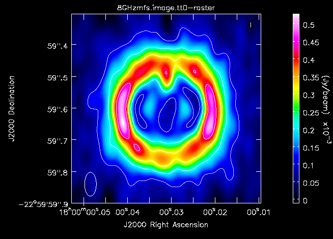
|
| This tutorial explains the steps for simulating VLA observations using the same protoplanetary disk sky model that was used for the analogous ALMA tutorial. Observational and analysis parameters are changed step by step and the results are compared to the VLA exposure calculator. | |
| Advanced: Corrupting Simulated Data (Simulator Tool) | |
| simobserve calls methods in the simulator tool. For advanced CASA users, the simulator tool has methods that can add to simulated data: phase delay variations, gain fluctuations and drift, cross-polarization, and bandpass and pointing errors. simulator also has more flexibility than simobserve in adding thermal noise. The tutorial linked from this page describes the simulation of data using the task interface only. The simulator tool is part of the CASA tool-kit. An examples of advanced techniques for corrupting a simulated MeasurementSet can be found in this CASA Guide on Corrupting Simulated Data (Simulator Tool). |
Archived Simulation Guides
This table includes past simulation guides which are no longer maintained.
Version History
For previous CASA versions, please see:
Simulating Observations in CASA 6
Simulating Observations in CASA 5.4
Simulating Observations in CASA 5.1
Simulating Observations in CASA 4.4
Simulating Observations in CASA 4.3
Simulating Observations in CASA 4.2
Simulating Observations in CASA 4.1
Simulating Observations in CASA 4.0
Simulating Observations in CASA 3.4
Simulating Observations in CASA 3.3
User Feedback
We welcome input on developing the CASA simulator. Contact https://help.almascience.org if you would like to volunteer your input.