Simulating ngVLA Data-CASA6.7.0
Introduction
The following tutorial shows how to create simulated data for the next generation Very Large Array (ngVLA). The configuration files for the different subarrays can be used for simulations and calculations that investigate the scientific capabilities of the ngVLA. Each configuration (.cfg) file contains the name of the observatory, the antenna positions, the coordinate system of the antenna positions and the diameter and pad name of each antenna. For these configuration files, the coordinate system is 'global', which signifies that the positions x, y, z are in meters relative to the Earth center following the FITS WCS convention.
CASA provides two ways to create a simulation: the simobserve task and the sm toolkit. With these methods we can generate measurement sets (MSs), add thermal noise, and predict model visibilities, from which we can explore the ngVLA’s imaging capabilities. The simobserve task is very user friendly but it is important to be aware that it has several limitations and it has been designed primarily for ALMA and the VLA. For this reason, we also demonstrate the use of the sm toolkit, which provides much more flexibility in setting the observational parameters and is more compatible with observatories that are not recognized by CASA.
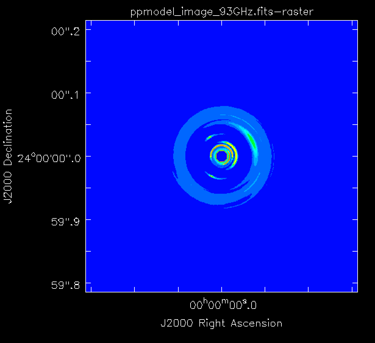
In this tutorial we present three example simulations: (i) simobserve using a model image, (ii) simobserve using a component list, and (iii) a sm toolkit simulation. For more information about component lists, refer to the Simulation Guide Component Lists and the Simulation Guide Component List for Selfcal. The model image used in portions of this guide, a 93 GHz model of a protoplanetary disk, is shown in Figure 1. Note that the pixel size of the model must correspond to the ngVLA longest baseline resolution at the requested frequency to work well. The next section will explain how to obtain the model image. We will also show how to create and use a component list instead of a model image for the simulations.
We will create example continuum simulations at 93 GHz, consisting of a single channel observed for a total of 4 hours with a 60 second correlator integration time† . We will then add to these simulations an amount of thermal noise that is representative of the ngVLA's continuum sensitivity. The array configuration used in this guide (Rev F) is the Main ngVLA subarray, which is composed of 214 18 m antennas and extends over a maximum baseline of ~1300 km. The next section will explain how to obtain this file.
† We choose this integration time in order to keep the MS files small. Time smearing is not an issue for simulated observations, but this value would need to be reconsidered before scheduling actual observations, e.g., on the order of 0.2 second correlator integration time.
Next Generation Very Large Array Configurations and Model Repository
ngVLA Configuration Files
The CASA data repository contains rry components for the ngVLA that can address different science goals depending on desired resolution. The components are listed in Tables 1 and 2; But any subarray antenna selection can be chosen independent of the components.
| Component Name | Aperture Diameter (m) | Quantity | Bmin (m) | Bmax (m) |
|---|---|---|---|---|
| Long Baseline Array | 18 | 30 | 495000 (38) | 8636000 |
| Main Interferometric Array | 18 | 214 | 42 | 1272600 |
| Short Baseline Array | 6 | 19 | 10.7 | 59.9 |
| Total Power/Single Dish | 18 | 4 | -- | -- |
| Sub-Component | Min. Baseline (m) | Max. Baseline (m) | Distribution Pattern | # Antennas |
|---|---|---|---|---|
| Core | 42 | 4272 | Constrained random | 114 |
| Spiral | 812 | 39270 | 5-arm spiral | 54 |
| Mid | 10120 | 1272600 | 5-arm spiral | 46 |
The data can be found at inside CASA under the path:
# In CASA
print(config.measurespath +'/alma/simmos')
which is frequently ~/.casa/data/alma/simmos or /home/casa/data/distro/alma/simmos/ at NRAO
The file that we use here is 'ngvla-revF.main.cfg' that is available at these paths.
For simplification, we copy the file to the current directory:
# In CASA
os.system('cp '+config.measurespath +'/alma/simmos/ngvla-revF.main.cfg .')
If the file is not available as described, the data repository needs to be updated. The following CASA command should do the trick, but we recommend to follow the instructions on CASA's External Data page.
# In CASA
!python3 -m casaconfig --update-all
!python3 -m casaconfig --current-data
Simulation Models
The model image used in portions of this guide is available at this link ppmodel_image_93GHz.fits.gz for direct download and will then need to be unzipped using gunzip, before using it in the simulations.
For additional models, please see the ngVLA model repository for currently available models.
Estimating the Scaling Parameter for Adding Thermal Noise
This section describes the procedure we will use to add noise to our simulations and the relevant calculations that we need to prepare for this. Simobserve's parameter to corrupt the simulated data is called thermalnoise and for interferometric data the allowed values are 'tsys-atm' , 'tsys-manual' or ' ' (refer to the Corrupting Simulated Data guide for more details). The option ' ' will not add any noise to the data, and the option 'tsys-atm' is only applicable to ALMA since it uses site parameters which are specific to that observatory. For the option 'tsys-manual' , it is necessary to supply several additional parameters which are required to construct an atmospheric model. In order to achieve the desired sensitivity without atmospheric modeling, we have chosen to corrupt the simulated data using the sm.setnoise function of the sm toolkit. In addition to the modes 'tsys-atm' and 'tsys-manual' , this function also allows the option of simplenoise. As the name indicates, simplenoise adds random Gaussian noise to the visibilities based on a simple scaling factor. We will use this same technique for all three example simulations, i.e., those made with the simobserve task and those made with the sm toolkit.
In order to estimate the scaling factor for the simplenoise parameter in sm.setnoise we use the following procedure:
The RMS noise ([math]\displaystyle{ \sigma_{NA} }[/math]) in an untapered, naturally-weighted Stokes I image will be approximately (see setnoise function) [math]\displaystyle{ \sigma_{NA} \sim \frac{\sigma_{simple}}{ \sqrt{n_{ch}\,n_{pol}\,n_{baselines}\,n_{integrations} }} }[/math] (1)
where [math]\displaystyle{ \sigma_{simple} }[/math] is the simplenoise parameter in sm.setnoise and corresponds to the noise per visibility, [math]\displaystyle{ n_{ch} }[/math] is the total number of channels across all spectral windows, [math]\displaystyle{ n_{pol} }[/math] is the number of polarizations used for Stokes I (typically 2) and [math]\displaystyle{ n_{integrations} }[/math] is the number of correlator integration times in the MS (i.e., total on-source time / integration time). For the example simulations in this guide, the track time is 4 hrs and the integration time is 60 sec, thus [math]\displaystyle{ n_{integrations}=240 }[/math]. Additionally, for these examples the total number of channels is 1 and the number of polarizations is 2. The number of baselines [math]\displaystyle{ n_{baselines} }[/math] is [math]\displaystyle{ N(N-1)/2 }[/math] where N is the number of antennas in the array. For the array configuration used in this guide (ngvla-revF.main.cfg), N=214 and therefore [math]\displaystyle{ n_{baselines}= 22791 }[/math].
If you already know the expected image noise ([math]\displaystyle{ \sigma_{NA} }[/math]) for your untapered, naturally-weighted image, you can solve for the scaling parameter [math]\displaystyle{ \sigma_{simple} }[/math] in the above equation (1) and pass [math]\displaystyle{ \sigma_{simple} }[/math] to the simplenoise parameter in sm.setnoise.
If instead you want to calculate the expected sensitivity for an ngVLA image, we suggest the following procedure:
(i) Calculate the expected untapered, naturally weighted point source sensitivity ([math]\displaystyle{ \sigma_{NA} }[/math]) using one of the ngVLA performance tables (see also the ngECT app). In Appendix D of ngVLA memo #55 there are key performance metrics for 6 subarrays which are tabulated as a function of frequency and resolution; the ngVLA Reference Design publication also has noise values in Table 6. For our example, we find in Table 10 of ngVLA memo #55 that the untapered, naturally weighted point source sensitivity of the Main interferometric array at 93 GHz is 0.83 uJy/beam for a 1 hour observation.
(ii) Scale that number to the desired observation length, in this case [math]\displaystyle{ t_{track}=4\,h }[/math]. Therefore, [math]\displaystyle{ \sigma_{NA} = 0.83/\sqrt{(t_{track}/1\,hour)} = 0.415\,\text{uJy/beam} }[/math].
(iii) Use the expected image noise ([math]\displaystyle{ \sigma_{NA} }[/math]) in the above equation (1) to solve for the scaling factor [math]\displaystyle{ \sigma_{simple} }[/math]. In this case, [math]\displaystyle{ \sigma_{simple}=0.415*\sqrt{1*2*22791*240} = 1.4\,\text{mJy} }[/math].
Once you have derived the scaling factor [math]\displaystyle{ \sigma_{simple} }[/math], run sm.setnoise and corrupt the visibilities of the noise-free MS. Your resulting untapered, naturally-weighted image will then have an RMS approximately equal to your desired image noise. Since it is not easy to undo this step, it is a good idea to make a copy of the noise-free MS before adding noise. The following mock example outlines this procedure:
# In CASA
## Create a copy of the noise-free MS:
os.system('cp -r noise_free.ms noisy.ms')

## Open the MS we want to add noise to with the sm tool:
sm.openfromms('noisy.ms')

## Set the noise level using the simplenoise parameter estimated earlier in this section:
sm.setnoise(mode = 'simplenoise', simplenoise = sigma_simple)

## Add noise to the 'DATA' column (and the 'CORRECTED_DATA' column if present):
sm.corrupt()

## Close the sm tool:
sm.done()
Note that this example will not execute without a MS named 'noise_free.ms' and a defined variable sigma_simple. See below for working examples of this procedure used in conjunction with the creation of simulated MSs and the prediction of model visibilities.
Example Simulation using Simobserve with a Model Image
We will use the simobserve task to create our first noise-free measurement set (MS), using the configuration file and model image described in the Introduction.
# In CASA

simobserve(project = 'ngVLA_214_ant_60s_noise_free-model',
                    skymodel = 'ppmodel_image_93GHz.fits',
                    setpointings = True,
                    integration = '60s',
                    obsmode = 'int',
                    antennalist = 'ngvla-revF.main.cfg',
                    hourangle = 'transit',
                    totaltime = '14400s',
                    thermalnoise = '',
                    graphics = 'none')
project: Simobserve will create a folder with the project name in your current working directory, and this folder will contain all the resulting files including the noise-free MS.
skymodel: The input model image in Jy/pixel units, can be a single image or a spectral cube. The simulated MS will inherit the number of channels, central frequency, source direction, and peak flux of this input model. These can be adjusted using the optional parameters inbright, indirection, incell, incenter, and inwidth. In this example, we do not modify these optional parameters.
setpointings: We choose the value of True, which allows simobserve to derive the pointing positions using its own algorithm and properties of the input model image. Since the size of the model is much smaller than the primary beam, a single pointing will be generated (instead of a mosaic). We also set the expanded parameter integration to '60s' (our chosen correlator integration time) and leave other expanded parameters set to their default values.
obsmode: We set this parameter to 'int' to simulate interferometric data. We also set values for several expandable parameters. For antennalist, we give the name of the configuration file for the ngVLA Main interferometric array. simobserve will read this file from a directory inside the CASA distribution (see the section on Obtaining the Necessary Files for this Guide). We set totaltime to the total on-source observation time, use the hourangle parameter to center our observation time on transit, and leave other expanded parameters as default.
thermalnoise: We leave this parameter empty to create a noise-free simulation. We will add the noise later in a separate step.
graphics: This will show graphics on the screen and/or save them as png files in the project directory. However, at the moment this is not working properly for baselines larger than a few hundred km. For this reason, we use 'none' in this example.
Now, to add thermal noise, we do the following:
# In CASA

## Create a copy of the noise-free MS:
os.system('cp -r ngVLA_214_ant_60s_noise_free-model/ngVLA_214_ant_60s_noise_free-model.ngvla-revF.main.ms  ngVLA_214_ant_60s_noisy-model.ms')

## Open the MS we want to add noise to with the sm tool:
sm.openfromms('ngVLA_214_ant_60s_noisy-model.ms')

## Set the noise level using the simplenoise parameter estimated in the section on Estimating the Scaling Parameter for Adding Thermal Noise:
sigma_simple = '1.4mJy'
sm.setnoise(mode = 'simplenoise', simplenoise = sigma_simple)

## Add noise to the 'DATA' column (and the 'CORRECTED_DATA' column if present):
sm.corrupt()

## Close the sm tool:
sm.done()
At this point, continue to imaging, or apply other manipulation steps to the MS.
Example Simulation using Simobserve with a Component List
Instead of using a model image we can use a component list for the simulation. Warning: At the moment, this method may take several times longer than using a model image due to internal issues with simobserve. Below is a simple example of how to make a component list consisting of a single point source.
# In CASA

## Position of the source that we want to observe:
direction = 'J2000 00:00:00.0 +24.00.00.0'

## Use the component list (cl) tool to make a model centered at the direction given above, and with a source flux of 10 uJy:
cl.addcomponent(dir = direction, flux = 10e-6, freq = '93GHz')

## Name of the component list model:
cl.rename(filename = 'my_component.cl')

## Close the component list:
cl.done()
More information on component lists can be found in the CASA documentation or in this small CASAguide example.
Now, we can use simobserve using the generated component list:
# In CASA

simobserve(project = 'ngVLA_214_ant_60s_noise_free-complist',
                    complist = 'my_component.cl' ,
                    compwidth = '10GHz',
                    setpointings = True,
                    integration = '60s',
                    obsmode = 'int',
                    antennalist = 'ngvla-revF.main.cfg',
                    hourangle = 'transit',
                    totaltime = '14400s',
                    thermalnoise = '',
                    graphics = 'none')
Most of the parameters are the same as the previous example. The parameters which are specific to using a component list are:
complist: Here we provide the component list created above. The expandable parameter compwidth indicates the bandwidth of the component, which will be used to set the bandwidth of the MS and resulting images.
Then we can add the thermal noise in the same way as in the section, Example Simulation using Simobserve with a Model Image.
Example Simulation using sm toolkit with either a Model Image or a Component List
# In CASA

## Set the name of the configuration file for the ngVLA Main subarray:
conf_file = 'ngvla-revF.main.cfg'


## Use simutil to read the .cfg file:
from casatasks.private import simutil
u = simutil.simutil()
xx,yy,zz,diam,padnames,antnames,observatory,measdict = u.readantenna(conf_file)


########################################################################
## Setting the observation framework, i.e., defining the sources,     ##
## resources, and scans similar to what we would do in the            ##
## Observation Preparation Tool (OPT) when setting up an observation. ##
########################################################################

## Simulate measurement set using the simulation utilities sm tool:
ms_name = 'ngVLA_214_ant_60s_noise_free.ms'     ## Name of your measurement set
sm.open( ms_name )

## Get the position of the ngVLA using the measures utilities (me):
pos_ngVLA = me.observatory('ngvla')

## Set the antenna configuration using the sm tool using the positions,
## diameter, and names of the antennas as read from the configuration file:
sm.setconfig(telescopename = observatory, x = xx, y = yy, z = zz,
                    dishdiameter = diam.tolist(), mount = 'alt-az',
                    antname = padnames, padname = padnames,
                    coordsystem = 'global', referencelocation = pos_ngVLA)

## Set the spectral windows, in this case, as a single channel.
## Simulation with a channel resolution of 10 GHz:
sm.setspwindow(spwname = 'Band6', freq = '93GHz', deltafreq = '10GHz',
freqresolution = '10GHz', nchannels = 1, stokes = 'RR RL LR LL')

## Set feed parameters for the antennas:
sm.setfeed('perfect R L')

## Set the field of observation that we are going to simulate
## (where the telescope is pointing), in this example we are using
## a Dec of +24deg.
sm.setfield(sourcename = 'My source',
                  sourcedirection = ['J2000','00h0m0.0','+24.0.0.000'])

## Set the limit of the observation for the antennas:
sm.setlimits(shadowlimit = 0.001, elevationlimit = '8.0deg')

## Weight to assign autocorrelation:
sm.setauto(autocorrwt = 0.0)

## Integration time or how often the array writes one visibility
## referencetime is the start date (today's date) and epoch measure ('utc'):
integrationtime = '60s'
sm.settimes(integrationtime = integrationtime, usehourangle = True,
            referencetime = me.epoch('utc', 'today'))

## Setting the observation duration, which for our example is 4 hrs
## because usehourangle=True above, these times are relative to HA=0:
starttime = '-2h'
stoptime = '2h'
sm.observe('My source', 'Band6', starttime = starttime, stoptime = stoptime)

## < steps for predicting model visibilities and adding noise can optionally appear here in this order >
## sm.predict...
## sm.setnoise...
## sm.corrupt...

## Close the simulator tool:
sm.close()
The above example will create a noise-free and source-free MS, which may be useful for certain studies (e.g., properties of the PSF). If desired, the steps to add sources and/or noise could be added to the above script after sm.observe or they can be run separately as in the examples below.
If we want sources in the field we can predict the visibilities using sm.predict function by providing either a CASA image or a component list.
Note the default behavior of sm.predict shown here will not include any attenuation by the antenna's primary beam. This may be fine for simulations of a compact source near the beam center, but not for wide-field simulations and mosaics. For more control over the predict step, see sm.setoptions or consider doing the visibility prediction using im.ft or tclean.
If using a component list, follow the steps below:
## Using the same component list that we generated in the section on Example Simulation using Simobserve with a Component List
## predicts the visibility of the source
sm.openfromms('ngVLA_214_ant_60s_noise_free.ms')
sm.predict( complist = 'my_component.cl')
sm.close()
However, if instead you want to use a model image, follow the steps below:
# In CASA

## To import the fits file as a CASA image:
model_file = 'ppmodel_image_93GHz'
importfits( fitsimage = model_file+'.fits', imagename = model_file+'.image')

## Note: A warning is produced in CASA when running importfits about the image not having a beam or angular resolution. This is expected since the model is in units of Jy/pixel and it can be safely ignored.

## To predict the model visibilities:
sm.openfromms('ngVLA_214_ant_60s_noise_free.ms')
sm.predict( imagename = model_file+'.image')

sm.close()
Note the model image should have units of Jy/pixel and not Jy/beam.
Finally, in order to add thermal noise, we do the following:
# In CASA

## Adding noise using the 'simplenoise' parameter estimated in the section on Estimating the Scaling Parameter for Adding Thermal Noise:
sigma_simple = '1.4mJy'
os.system('cp -r ngVLA_214_ant_60s_noise_free.ms ngVLA_214_ant_60s_noisy.ms')
sm.openfromms('ngVLA_214_ant_60s_noisy.ms')
sm.setnoise(mode = 'simplenoise', simplenoise = sigma_simple)
sm.corrupt()
sm.done()
Comparison of the Results with the Expected Image Noise
Here we will create an image to confirm that the noise we added is as expected, using the simulated MS created in the section, Example Simulation using Simobserve with a Model Image.
In order to determine an appropriate cell size we use im.advise, a helper function which suggests recommended values of certain imaging parameters. The third value returned by im.advise is the maximum cell size that will allow the longest baselines to be gridded. We want to avoid using a value larger than this maximum size to ensure that all the data is used during imaging.
# In CASA

im.open('ngVLA_214_ant_60s_noisy-model.ms')
print( im.advise() )
im.close()
For this MS, im.advise gives a value of 0.000282 arcseconds which we round to 0.3 mas. We then choose an image size of 3000 pixels in order to have a field of view comparable to our original model image.
Since it will be difficult to accurately measure the image noise with the source present, we can arrange for tclean to subtract the model and image only the residual visibilities. We will do this by setting the tclean startmodel parameter to that of our model image.
# In CASA
# If the model has not been converted from fits to CASA, then do the following, otherwise skip the next line:
importfits( fitsimage = 'ppmodel_image_93GHz.fits', imagename = 'ppmodel_image_93GHz.image')

#Make the image
tclean(vis = 'ngVLA_214_ant_60s_noisy-model.ms', datacolumn = 'data', imagename = 'sm_clean_noisy', imsize = 2560, cell = '0.3mas',  startmodel = 'ppmodel_image_93GHz.image', specmode = 'mfs',  gridder = 'standard', deconvolver = 'hogbom', weighting = 'natural', niter = 0)
A different method would be to set the image to zero in immath, then repeat the same https://casadocs.readthedocs.io/en/v6.7.0/api/tt/casatasks.simulation.simobserve.html simobserve] step as above and add the noise. This image has no emission an[d should represent the noise only.
We can then open the residual image in the CARTA visualization program:
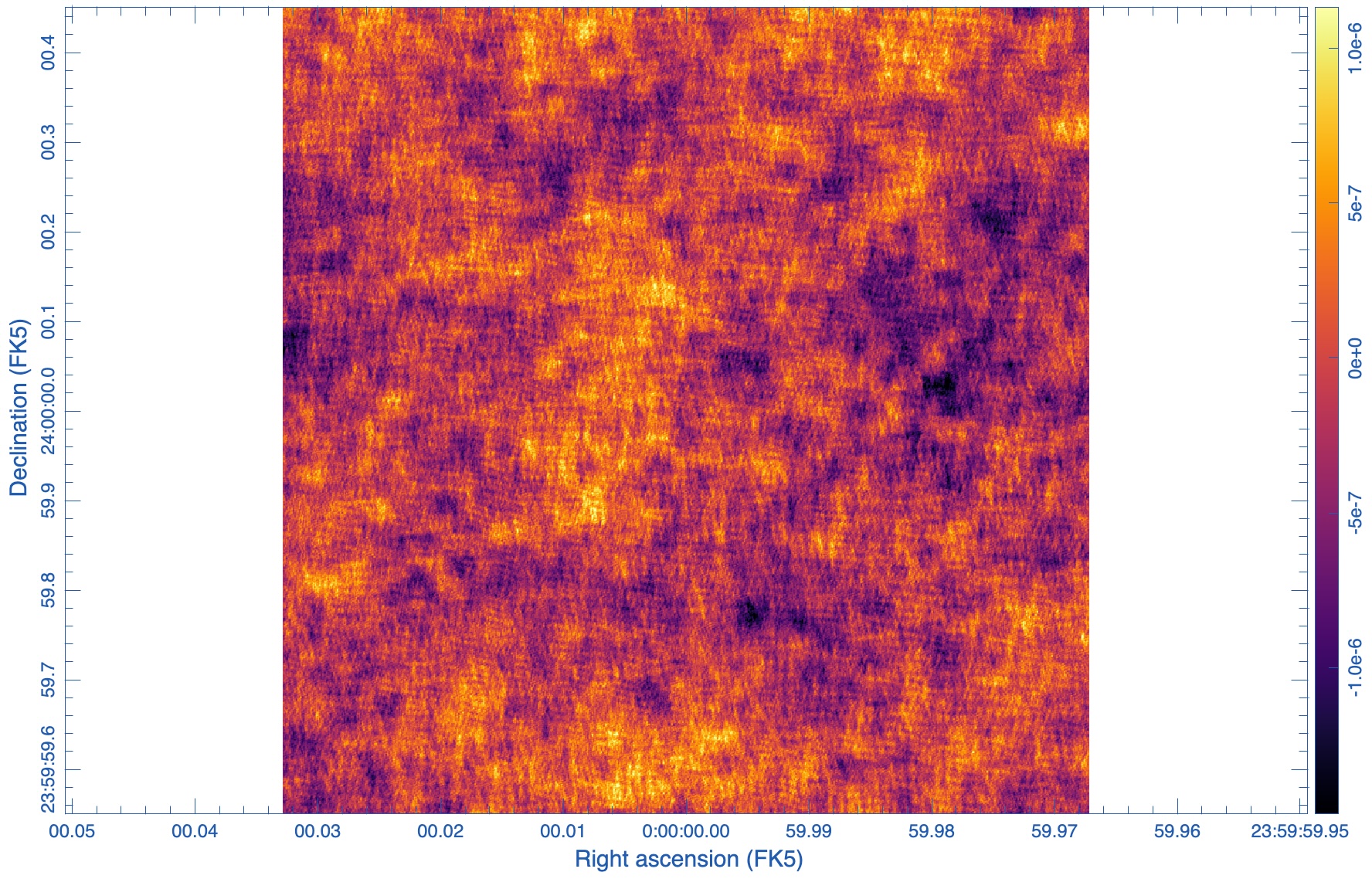
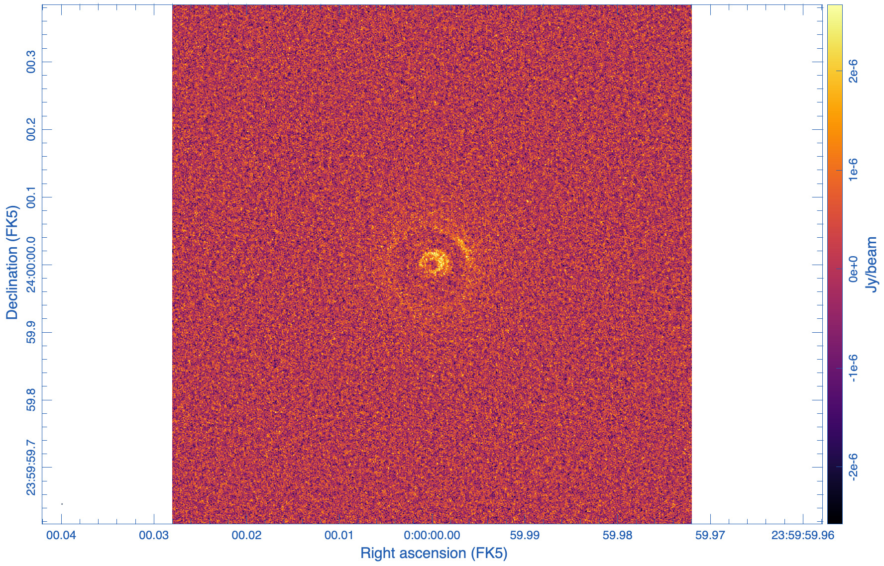
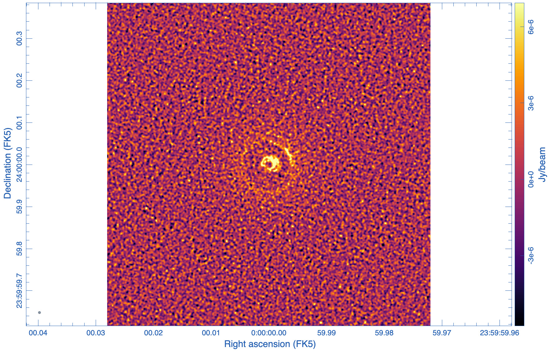
Figure 2 shows our residual image. The noise pattern in your image may look different since each execution of sm.corrupt will generate different random numbers, but the RMS should be very similar. Since we have subtracted the same model that we used to predict the source visibilities, the residual image will contain only on the noise we added with 'simplenoise' . This residual image is essentially equivalent to the image you would get for a simulation without any sources in the field.
 |
The image statistics, and in particular the rms noise statistics, can be called like:
# In CASA
stat=imstat('sm_clean_noisy.residual')
print(stat['rms'])
[4.28513655e-07]
Alternatively, the statistics widget in CARTA can be used.
The value should be of similar order, but given the randomness of noise it will not be identical to the one above.
The image RMS is in good agreement with the expected image RMS of 0.415 uJy/beam from the section on Estimating the Scaling Parameter for Adding Thermal Noise.
Imaging
The ngVLA is not reconfigurable. Hence, the configuration has been designed to capture information on scales of arcminutes (SBA) to sub-milliarcseconds (LONG). As such, when using eg. all antennas in MAIN (Core+SPIRAL+Mid), baselines are sampled from 40 m to 1000 km. Further, the relative weighting, with Core having half the collecting area within 2km radius, leads to a PSF with essentially three scales: a very narrow spike from Mid antennas, a first skirt due to the Spiral, and a very broad second skirt due to Core. Numerous studies have been done that balance tapering and Briggs weighting to achieve better behaved PSFs (see ngVLA memo #65, #92 ngVLA). Ultimately, the ngVLA will operate with subarrays, with subsets of antennas selected based on the science goals (see ngVLA memo #121).
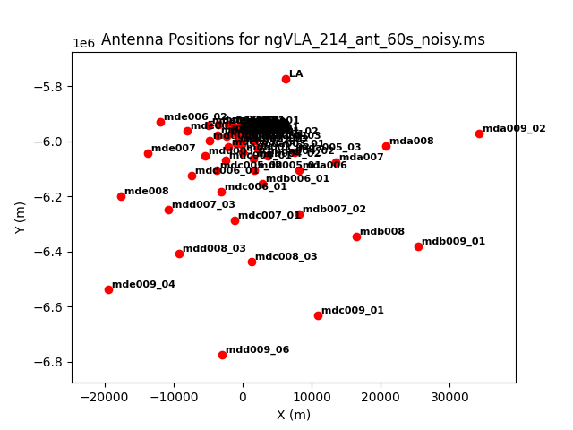
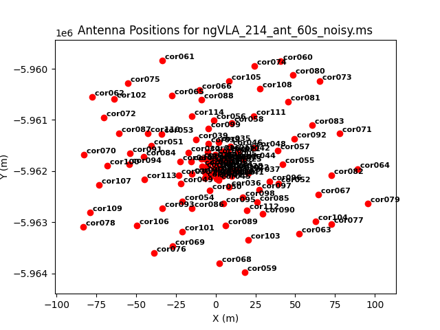
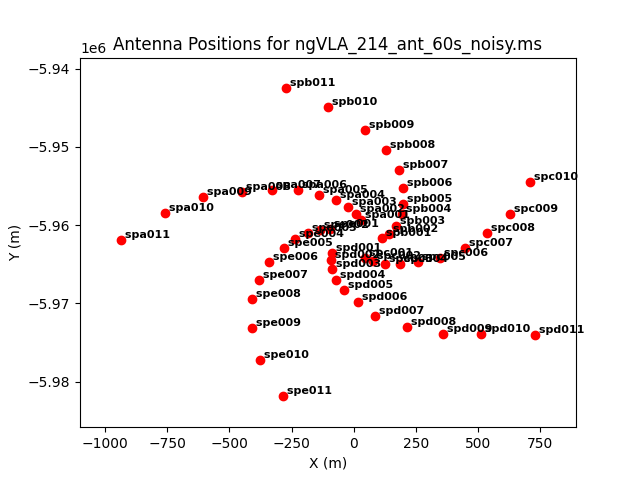
As an example, we image the MS that was created with the model image. Let's first get an overview of the complex antenna positioning of the ngVLA (Fig. 3), we will plot the main array used in this simulations, and the different sub-components (core, spiral, and mid arrays; main array = core+spiral+mid).
# In CASA
plotants(vis='ngVLA_214_ant_60s_noisy-model.ms')
plotants(vis='ngVLA_214_ant_60s_noisy-model.ms',exclude='md*,LA,sp*')
plotants(vis='ngVLA_214_ant_60s_noisy-model.ms',exclude='md*,LA,co*')
plotants(vis='ngVLA_214_ant_60s_noisy-model.ms',exclude='sp*,LA,co*')
 |
 |
 |
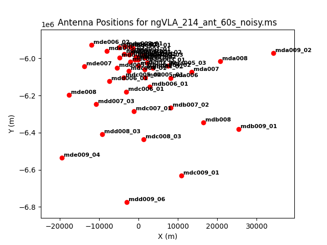 |
The different areas and antenna densities are obvious (compare the different scaling on the axes).
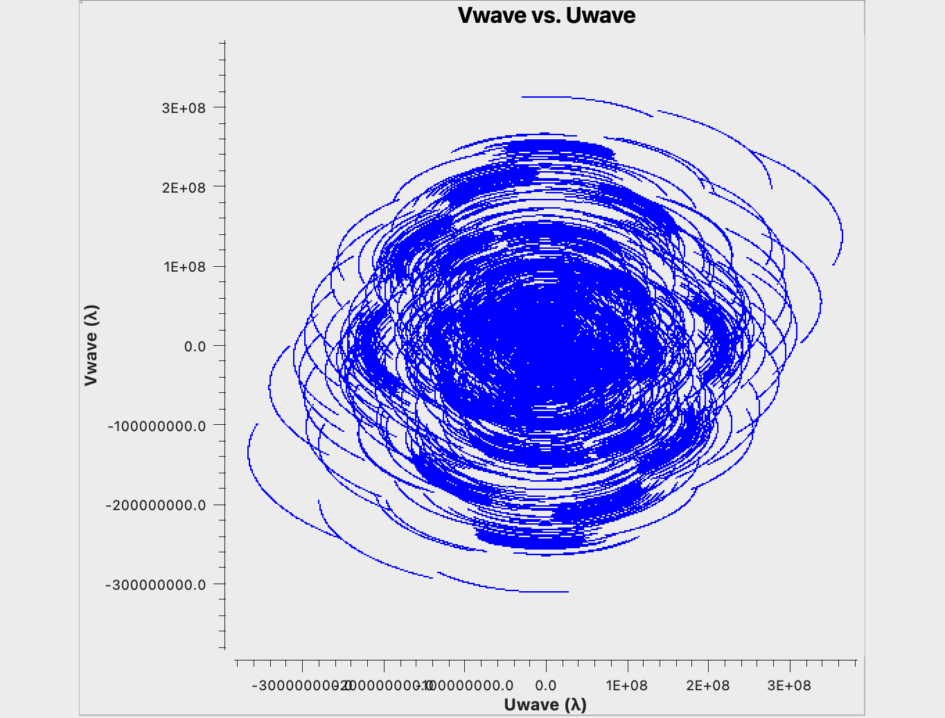
For the purpose of our model dataset, aperture synthesis creates the uv-coverage shown in Fig. 4:
# In CASA
# plot the uv coverage for a single channel to speed things up.
plotms(vis='ngVLA_214_ant_60s_noisy-model.ms', spw='0:1',xaxis='uwave',yaxis='vwave')
plotms(vis='ngVLA_214_ant_60s_noisy-model.ms', spw='0:1',xaxis='uwave',yaxis='vwave',plotrange=[-1e6,1e6,-1e6,1e6])
 |
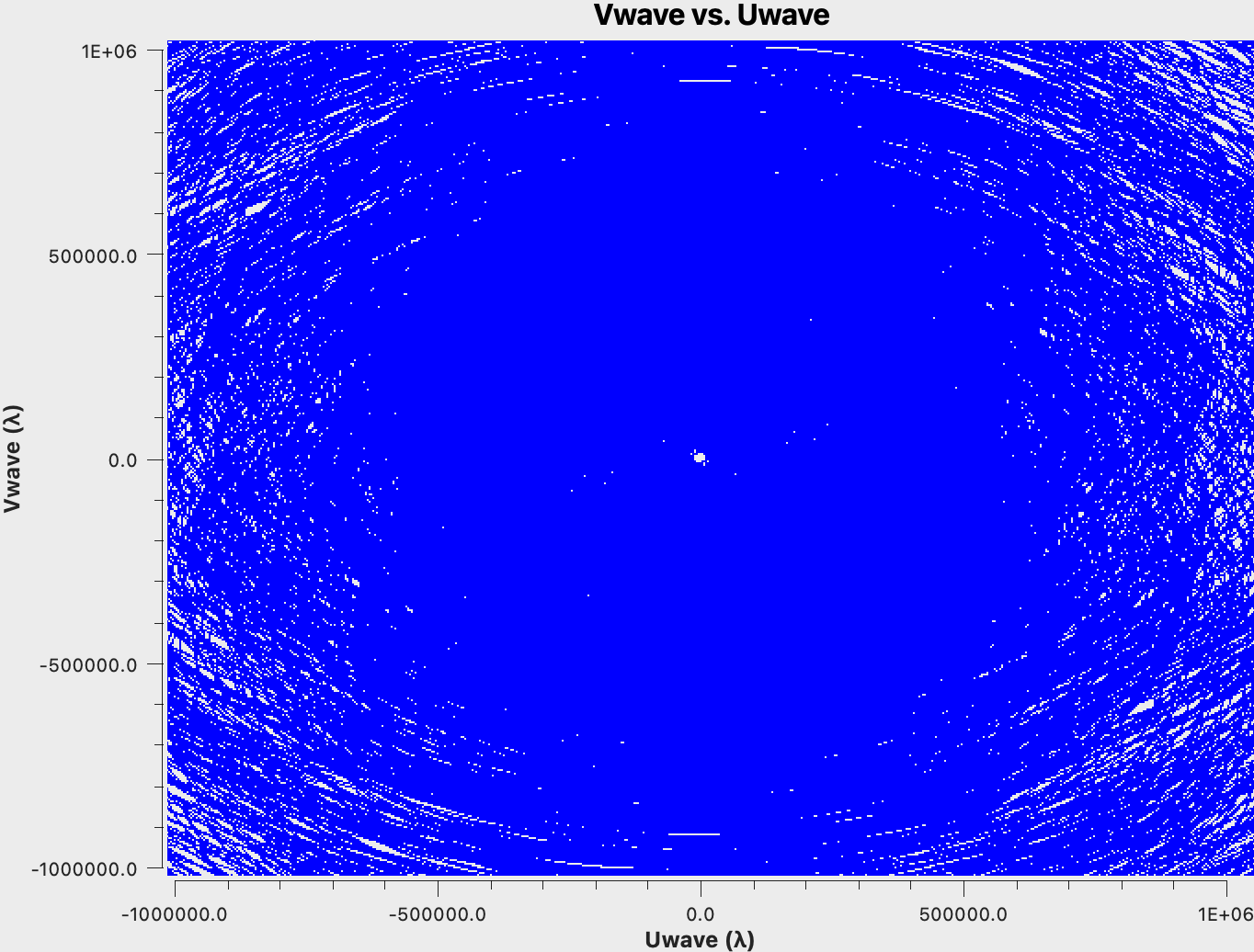 |
As expected, the uv-coverage is dense in the center and more sparse further out, which is the root of the challenges for the optimum weighting of the data. We would also like to point out the hole in the uv-coverage at near u=v=0. These are the short and zero spacings responsible for the largest scales in the image. The SBA (short baseline array) and/or a single dish is needed to image those and to fill the uv hole (cf. ngVLA memo #67, and ngVLA memo #89. The ngVLA SBA antenna configuration is also available on the ngVLA Configuration Tools webpage. Furthermore, for our small image of 0.8", the shorter baselines of the ngVLA core contribute less to the image; they would be more pronounced for larger fields.
In the following we will first test the parameter space by creating images with Briggs robust=-1, 0, and +1 weighting, which explores the parameter space from slightly uniform to slightly natural weighting.
# In CASA
tclean(vis='ngVLA_214_ant_60s_noisy-model.ms', datacolumn='data', imagename='ppdisk-sim-rob-1', imsize=2560, cell='0.3mas', specmode='mfs', weighting='briggs', robust=-1, niter = 10000, threshold='1e-5Jy')

tclean(vis='ngVLA_214_ant_60s_noisy-model.ms', datacolumn='data', imagename='ppdisk-sim-rob0', imsize=2560, cell='0.3mas', specmode='mfs', weighting='briggs', robust=0, niter = 10000, threshold='5e-6Jy')

tclean(vis='ngVLA_214_ant_60s_noisy-model.ms', datacolumn='data', imagename='ppdisk-sim-rob1', imsize=2560, cell='0.3mas', specmode='mfs', weighting='briggs', robust=1, niter = 10000, threshold='3e-6Jy')
 |
 |
 |
 |
 |
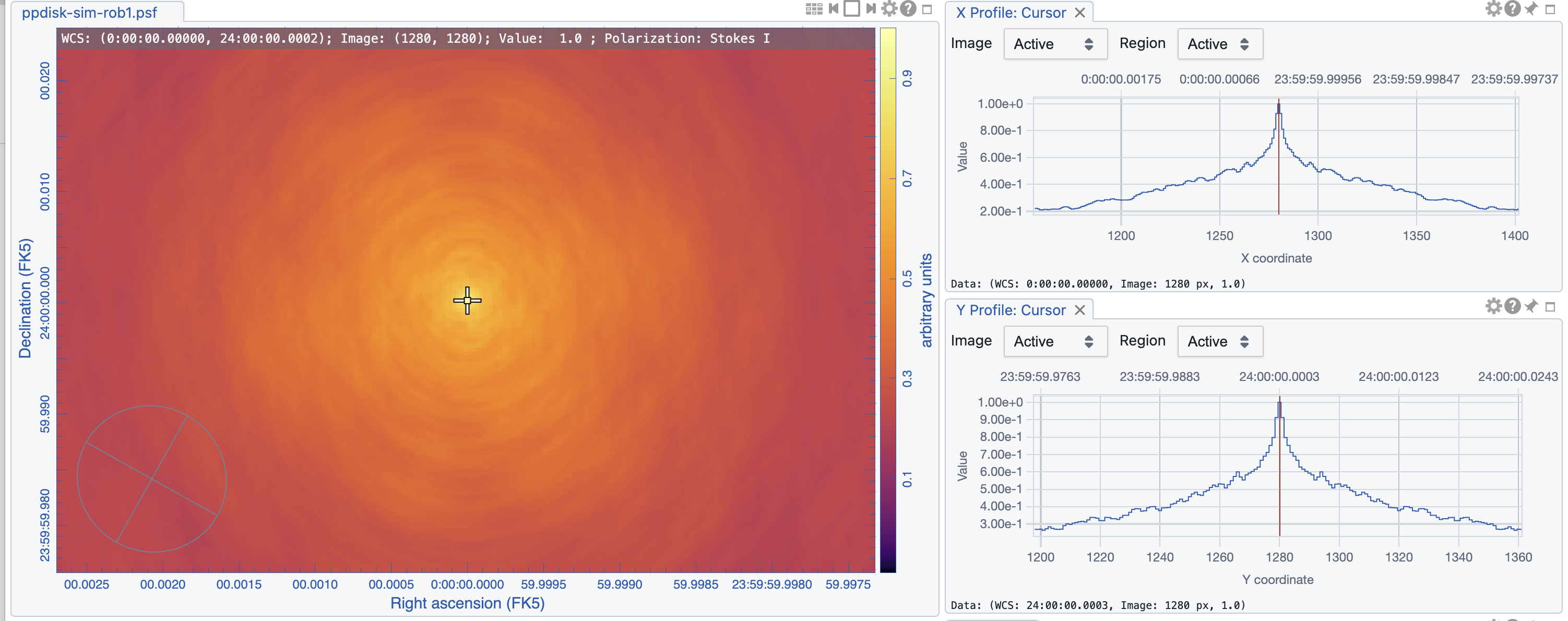 |
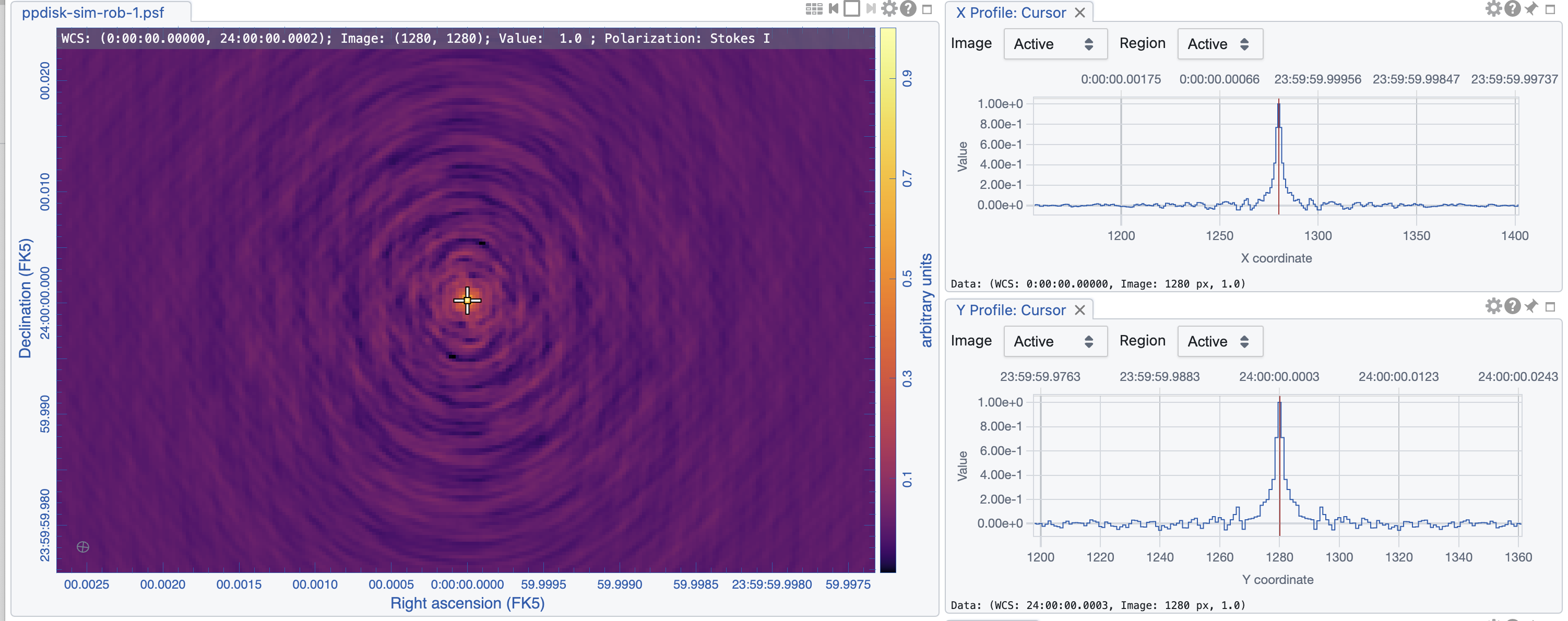
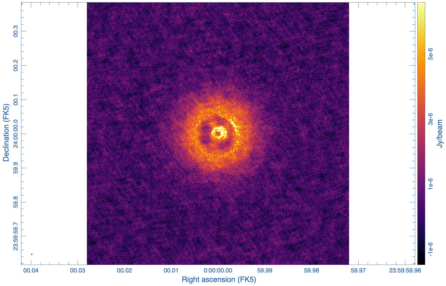
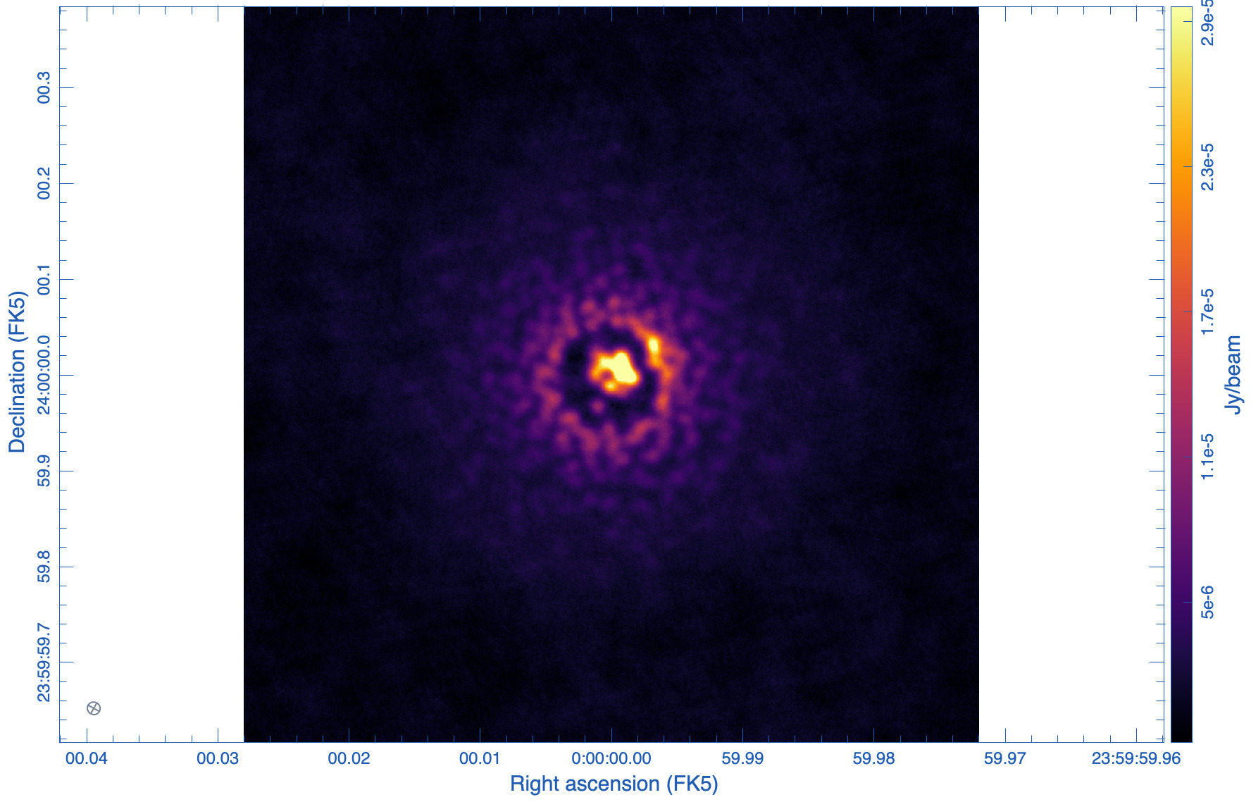
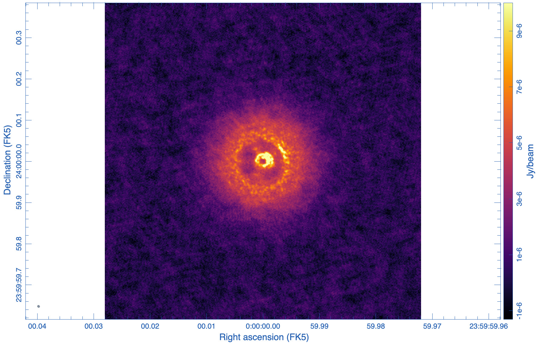
The images are shown in Figs. 5, 6, and 7. As expected, the lowest robust parameter of -1 is a weighting that emphasizes the longer uv-distances, shows higher resolution and larger noise. The robust=1, on the other hand, is emphasizing the shorter baselines and has a better sensitivity, traded for a larger beam. The associated beams, however, have very different shapes: Due to the dense ngVLA core followed by a less dense distribution on intermediate baselines, the psf is extremely sensitive on the Briggs weighting with very large wings for positive robust values (more natural) and more Gaussian for negative values (more uniform).
Let's numerically evaluate this:
# In CASA
for i in ['-1','0','1']:
 stat=imstat(imagename='ppdisk-sim-rob'+str(i)+'.image',box='0,0,200,200')
 head=imhead(imagename='ppdisk-sim-rob'+str(i)+'.image')
 print('ppdisk-sim-rob'+str(i)+'.image:'+' rms: '+str(stat['rms'])+'; bmaj: '+str(head['restoringbeam']['major'])+'; bmin: '+str(head['restoringbeam']['minor'])+'\n')
ppdisk-sim-rob-1.image: rms: [8.38892296e-07]; bmaj: {'unit': 'arcsec', 'value': 0.0010262896539643407}; bmin: {'unit': 'arcsec', 'value': 0.0009305544081144035}

ppdisk-sim-rob0.image: rms: [5.41353392e-07]; bmaj: {'unit': 'arcsec', 'value': 0.00339712668210268}; bmin: {'unit': 'arcsec', 'value': 0.003354895394295454}

ppdisk-sim-rob1.image: rms: [4.02055656e-07]; bmaj: {'unit': 'arcsec', 'value': 0.013521017506718636}; bmin: {'unit': 'arcsec', 'value': 0.013068420812487602}
Again, your values should be similar but not identical given the randomness of noise.
The robust=-1 has a rms of only about 30% more than the robust=0 image, but that is enough to make the emission less visible. The resolution of the robust=1 image, on the other hand, has a resolution twice that of robust=0 (in linear terms). So the robust=0 image is a compromise of sensitivity and resolution, but it still shows extended wings where a Gaussian approximation might not be the right choice.
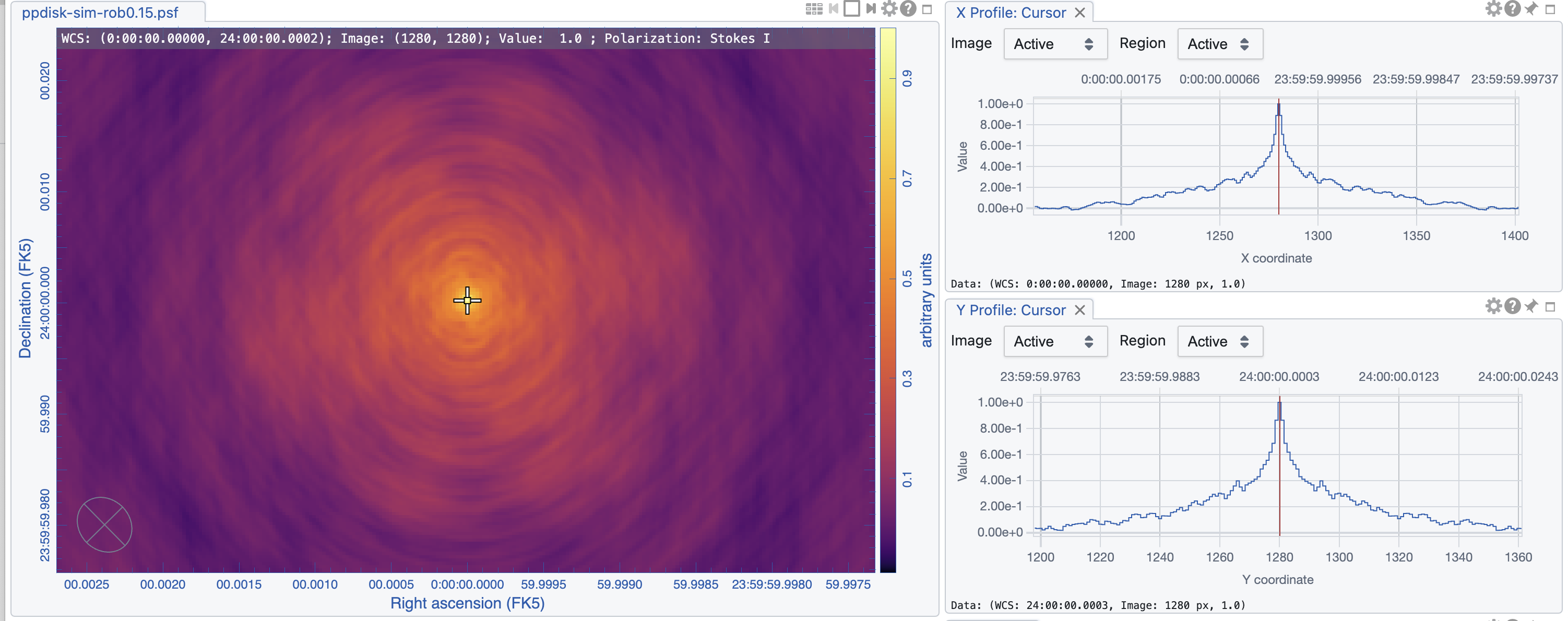
To demonstrate this effect, we now try to achive a 5mas beam in two ways: a) with a robust=0.15 parameter and b) following ngVLA memo #121 KSP-1, using robust=-1.81 and a taper of 4.68mas:
# In CASA

tclean(vis='ngVLA_214_ant_60s_noisy-model.ms', datacolumn='data', imagename='ppdisk-sim-rob0.15', imsize=2560, cell='0.3mas', specmode='mfs', weighting='briggs', robust=0.15, niter = 10000, threshold='6e-6Jy')

tclean(vis='ngVLA_214_ant_60s_noisy-model.ms', datacolumn='data', imagename='ppdisk-sim-rob-1.81-taper4.68mas', imsize=2560, cell='0.3mas', specmode='mfs', weighting='briggs', robust=-1.81, niter = 10000, threshold='1.5e-5Jy',uvtaper=['4.68mas','4.68mas','0deg'])


for i in ['0.15','-1.81-taper4.68mas']:
 stat=imstat(imagename='ppdisk-sim-rob'+str(i)+'.image',box='0,0,200,200')
 head=imhead(imagename='ppdisk-sim-rob'+str(i)+'.image')
 print('ppdisk-sim-rob'+str(i)+'.image:'+' rms: '+str(stat['rms'])+'; bmaj: '+str(head['restoringbeam']['major'])+'; bmin: '+str(head['restoringbeam']['minor'])+'\n')
ppdisk-sim-rob0.15.image: rms: [5.20132407e-07]; bmaj: {'unit': 'arcsec', 'value': 0.0052693807519972324}; bmin: {'unit': 'arcsec', 'value': 0.004550443962216377}

ppdisk-sim-rob-1.81-taper4.68mas.image: rms: [1.790868e-06]; bmaj: {'unit': 'arcsec', 'value': 0.005246456246823072}; bmin: {'unit': 'arcsec', 'value': 0.004973555449396372}
 |
 |
 |
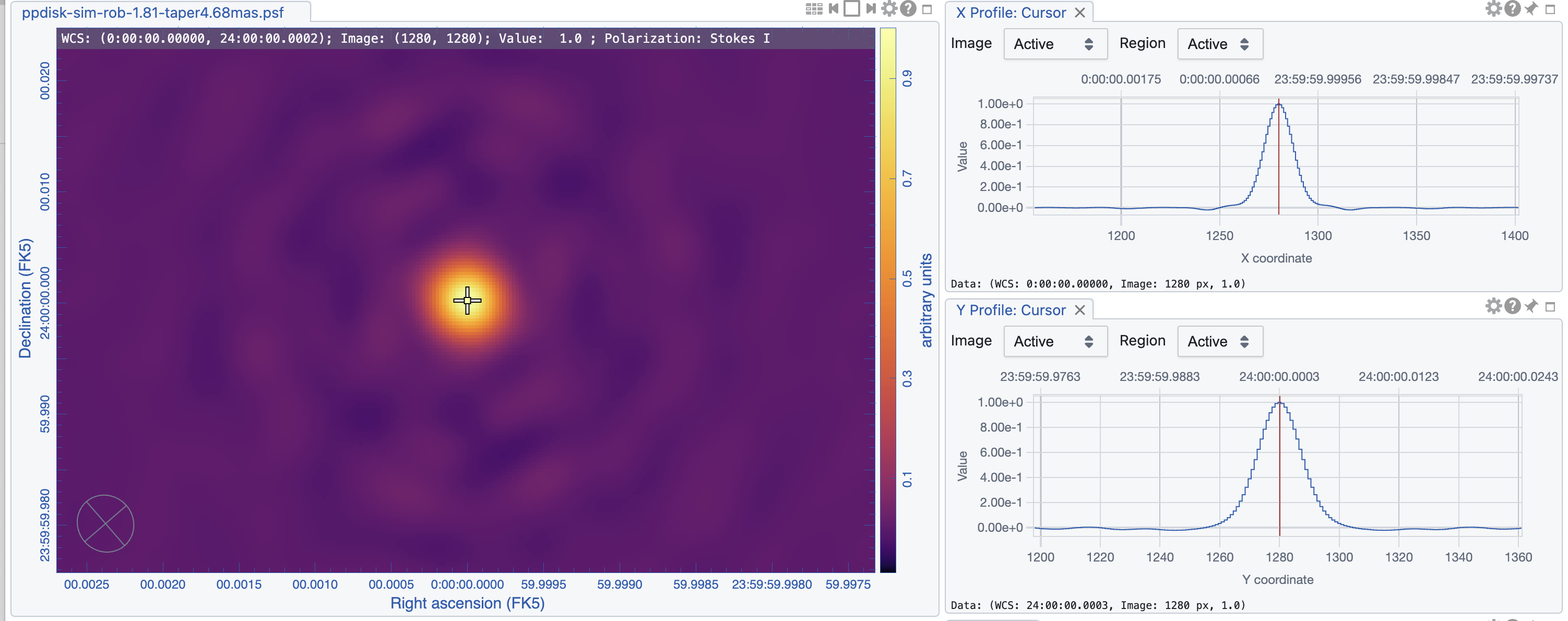 |
The statistics is showing that the beams for the two images are similar in size, 5mas, as designed. The psf wings, however, are substantially larger for the robust=0.15 image (cf. Figs 8, 9). High dynamic range imaging may therefore be problematic as to deconvolve bright, extended emission. The rms, however, is much improved with robust=0.15, as no tapering was needed and all antennas contribute to the overall sensitivity.
In the end, the scientific question dictates whether the image should have a high resolution or high surface brightness sensitivity, and we refer to ngVLA memos #65 for the old, revC ngVLA configuration; see also ngVLA memos #55, #76, #92, #105, and #121.
We also like to point out, that the above imaging is only for quick views. Improved imaging and deconvolution methods include multi-frequency synthesis, multi-scale clean, widefield and A projection, self-calibration and other calibration and imaging refinements, spectral line and polarization requirements, image combination with single dish data, etc. The scientific requirement and type of model will define the needed techniques, similar to current ALMA or VLA data.
Last checked on CASA Version 6.7.0.