Imaging an EVLA OSRO HI data set: Difference between revisions
No edit summary |
No edit summary |
||
| Line 57: | Line 57: | ||
* '''Y Axis''' = Amp | * '''Y Axis''' = Amp | ||
The figure to the right shows the resulting plot in [[plotms]]. There is clearly some line emission around channel 190, and possibly some faint emission around channel 85. Let's use channels | The figure to the right shows the resulting plot in [[plotms]]. There is clearly some line emission around channel 190, and possibly some faint emission around channel 85. Let's use channels 10--55 and 120--155 to fit the continuum. | ||
</div> | </div> | ||
| Line 67: | Line 67: | ||
|} | |} | ||
[[Main Page | ↵ '''CASA Guides''']] | [[Main Page | ↵ '''CASA Guides''']] | ||
Revision as of 00:32, 12 March 2010
This article is under construction. Watch this space!
Overview
This tutorial explains how to image an HI dataset acquired with the WIDAR0 correlator. It assumes that you've already calibrated your data as described in the calibration tutorial, and that you now have a split dataset with a single source of interest in it. In this example, the source is called 'Leo-2'; see the calibration tutorial for more details on this data set.
Flag Your Split Data
Load the split dataset into plotms and/or viewer and flag any bad data.
For a spectral line dataset like this one, you'll probably want to average in various ways to spot bad data. Averaging channels together can make bad baselines pop up!
Doppler Tracking
Presently, doppler tracking is not performed online by the EVLA, so we have to correct for any velocity shifts now, in post-processing, with cvel.
#  cvel :: regrid an MS to a new spectral window / channel structure or frame
vis                 =  'leo2.ms'        #  Name of input measurement set
outputvis           = 'leo2_cvel.ms'    #  Name of output measurement set
passall             =      False        #  Pass through (write to output MS) non-selected data with no change
field               =         ''        #  Select field using field id(s) or field name(s)
spw                 =        '0'        #  Select spectral window/channels
selectdata          =      False        #  Other data selection parameters
mode                =  'channel'        #   Regridding mode
     nchan          =         -1        #  Number of channels in output spw (-1=all)
     start          =          0        #  first input channel to use
     width          =          1        #  Number of input channels to average
     interpolation  =   'linear'        #  Spectral interpolation method

phasecenter         =         ''        #  Image phase center: position or field index
restfreq            = '1420405751.786Hz' #  rest frequency (see help)
outframe            =     'BARY'        #  Output frame (''=keep input frame)
veltype             =    'radio'        #  velocity definition
hanning             =      False        #  Turn on Hanning smoothing of spectral channels
async               =      False        #  If true the taskname must be started using cvel(...)
Cvel creates a new measurement set (outputvis= 'leo2_cvel.ms') for which, at each time, the spectrum has been shifted and channels regridded to keep the spectral line centered in the frame of your choice (here, we choose barycentric; outframe= 'BARY'). You'll also want to give cvel the rest frequency of your spectral line (restfreq= '1420405751.786Hz' for HI).
Continuum Subtraction
|
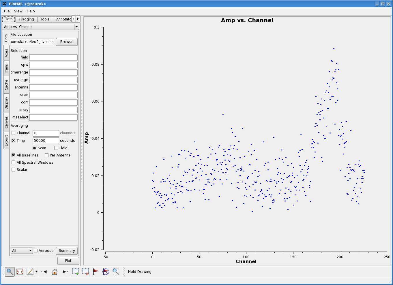
In preparation for subtracting the continuum, let us plot up the combined spectrum on our science field and identify some line-free channels. Open up a plotms GUI window and load the doppler-tracked measurement set containing your science target. You'll want to average over both time and baselines to get as much signal-to-noise as possible, hopefully revealing a nice 21 cm profile. In the Data tab of plotms, set the below averaging options:
(See Averaging data in plotms for more details on averaging options). You'll also want to click on the Axes tab in the plotms window, and change the axes settings to:
The figure to the right shows the resulting plot in plotms. There is clearly some line emission around channel 190, and possibly some faint emission around channel 85. Let's use channels 10--55 and 120--155 to fit the continuum. |
