Guide To Simulating ALMA Data: Difference between revisions
| Line 34: | Line 34: | ||
{| style="width: 100%; valign: top; background-color:#E0E0E0; border:1px solid #3366FF; text-align: left; cellpadding=0" | {| style="width: 100%; valign: top; background-color:#E0E0E0; border:1px solid #3366FF; text-align: left; cellpadding=0" | ||
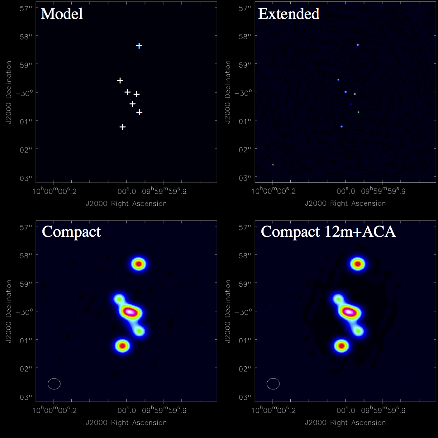
| rowspan=2; stype="border-bottom:1px solid black;" | [[File: | | rowspan=2; stype="border-bottom:1px solid black;" | [[File:Points-panels-hf.png | 200px]] | ||
! A Collection of Point Sources | ! A Collection of Point Sources | ||
|- | |- | ||
| Line 46: | Line 46: | ||
{| style="width: 100%; valign: top; background-color:#E0E0E0; border:1px solid #3366FF; text-align: left; cellpadding=0" | {| style="width: 100%; valign: top; background-color:#E0E0E0; border:1px solid #3366FF; text-align: left; cellpadding=0" | ||
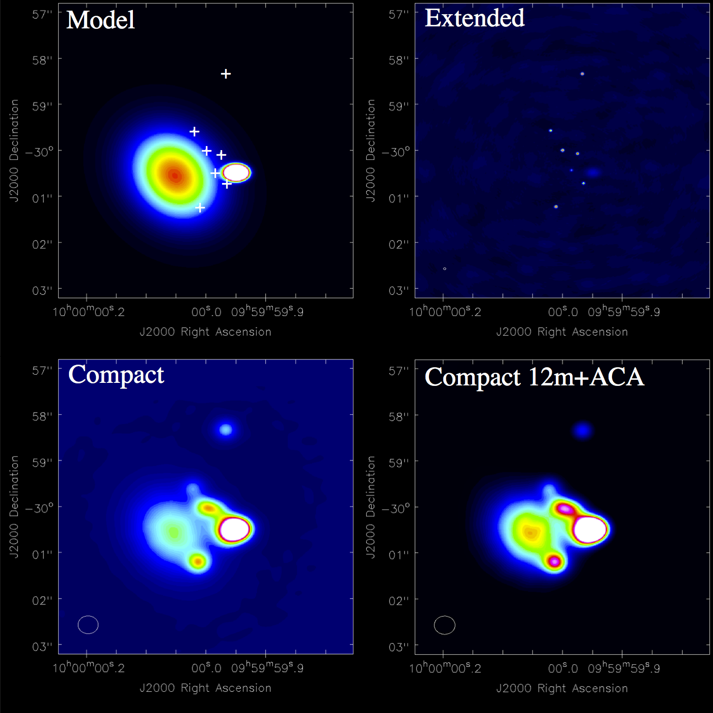
| rowspan=2; stype="border-bottom:1px solid black;" | [[File: | | rowspan=2; stype="border-bottom:1px solid black;" | [[File:Gaussians-panels-hf.png | 200px]] | ||
! Point Sources and Elliptical Gaussian Brightness Distributions | ! Point Sources and Elliptical Gaussian Brightness Distributions | ||
|- | |- | ||
| Line 58: | Line 58: | ||
{| style="width: 100%; valign: top; background-color:#E0E0E0; border:1px solid #3366FF; text-align: left; cellpadding=0" | {| style="width: 100%; valign: top; background-color:#E0E0E0; border:1px solid #3366FF; text-align: left; cellpadding=0" | ||
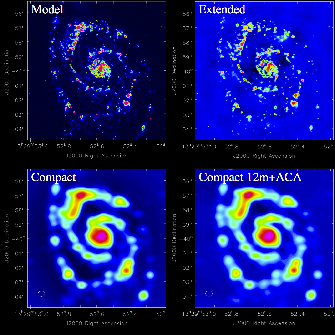
| rowspan=2; stype="border-bottom:1px solid black;" | [[File: | | rowspan=2; stype="border-bottom:1px solid black;" | [[File:M51-panels-hf.png | 200px]] | ||
! An M51-like Galaxy | ! An M51-like Galaxy | ||
|- | |- | ||
| style="border-bottom:1px solid black;" | Here we simulate an observation of a galaxy similar to M 51 | | style="border-bottom:1px solid black;" | Here we simulate an observation of a galaxy similar to M 51. | ||
|- | |- | ||
|} | |} | ||
--- | --- | ||
<!-- | <!-- comment this out? --> | ||
{| style="width: 100%; valign: top; background-color:#E0E0E0; border:1px solid #3366FF; text-align: left; cellpadding=0" | {| style="width: 100%; valign: top; background-color:#E0E0E0; border:1px solid #3366FF; text-align: left; cellpadding=0" | ||
| rowspan=2; stype="border-bottom:1px solid black;" | [[File: | | rowspan=2; stype="border-bottom:1px solid black;" | [[File:Proto-panels-hf.png | 200px]] | ||
! A Simplified Model of a Proto-planetary Disk | ! A Simplified Model of a Proto-planetary Disk | ||
|- | |- | ||
| style="border-bottom:1px solid black;" | This simulation shows a ring plus a planet | | style="border-bottom:1px solid black;" | This simulation shows an observation of a model image representing a ring plus a planet. | ||
|- | |- | ||
|} | |} | ||
--> | <!-- comment this out? --> | ||
== ALMA Simulation Tools == | == ALMA Simulation Tools == | ||
Revision as of 20:11, 23 October 2013
THIS PAGE IS UNDER CONSTRUCTION
Introduction: About this Document
This document describes why and how to use simulated observations to help understand your ALMA data, or to help you plan an ALMA observation. The document covers:
- Why you might want to simulate ALMA observations
- How simulations can help you plan a proposal
- Examples of simulating ALMA data
- Running your own simulations with the ALMA Observation Support Tool
- Simulating ALMA observations with CASA sim tools (using CASA 4.2)
Why Simulate ALMA Observations?
Observations made with radio interferometers can be tricky to interpret and analyze. Interferometers do not sample all spatial frequencies on the sky, so the image you generate from an interferometric observation does not necessarily represent the full sky brightness distribution. Specifically, interferometers are not sensitive to diffuse emission, and depending on a number of factors including the placement of the individual antennas, the length of the observation, and the location of the target source on the sky, an interferometric observation will be insensitive to structure on some angular scales. Observers therefore should use care when analyzing and interpreting interferometric images.
Plots of "uv coverage" are often used to illustrate the range of spatial frequencies measured by a specific interferometric observation. A uv coverage plot can be thought of as a mask that is applied to the Fourier transform of the emission pattern on the sky. More densely sampled uv coverage leads to better images because the observation is more sensitive to a wider range of spatial frequencies on the sky.
Several interferometers, including ALMA and the VLA, offer a number of antenna configurations, amounting to a "zoom lens" capability. To aid in interpreting their data, observers may find it helpful to simulate an interferometric observation using a variety of antenna configurations and different models of the sky brightness distribution. Simulations can also be a powerful tool to help new users understand both the power and the limitations of interferometric observations.
A Note Regarding Use of ALMA Simulations in your Proposal
Simulations of ALMA observations are not required for an ALMA proposal; however, a simulation could bolster an ALMA proposal in some cases. For example, simulations can demonstrate the need for specific configurations, or combinations of configurations, to resolve certain structures or meet specific scientific goals.
In Full Operations, ALMA will include a main array of fifty 12-m antennas, and the ALMA Compact Array (ACA) which encompasses twelve 7-m antennas and four 12-m antennas used for "total power" observations. At this time, every ALMA observation employs the 12-m main array. The 7-m array and Total Power observations are optional, used to fill in large-scale structure in mapping experiments. The ALMA OT advises users on whether to use the ACA based on two numbers: the required resolution and the maximum angular scale. If you have some uncertainty in the spatial scales for your ALMA target, you may wish to use simulations to justify inclusion of the ACA.
Background Information for Those New to Interferometry
Those new to interferometric observing can gain some intuition on the use of interferometers by exploring several software tools available on the web. For example, the Virtual Radio Interferometer is an interactive java application that allows one to simulate basic observations with MERLIN, ATCA, or WSRT, or ASKAP. The VRI can demonstrate how antenna arrangement affects uv coverage, the synthesized beam (i.e. the "resolution"), and the range of spatial sensitivities. Users can select from a few sample, idealized sky brightness patterns (e.g. a narrow gaussian) or use real sky images, then fiddle interactively with the placement of antennas and the duration of the observation to see the effects of uv coverage on observations.
Sample Simulations
Before getting to the details of using ALMA simulation tools, it is useful to examine a few example simulations. These examples were generated with the CASA simulation software described later in this document. These simulations demonstrate how observing with different ALMA configurations can affect the final image.
---
---

|
An M51-like Galaxy |
|---|---|
| Here we simulate an observation of a galaxy similar to M 51. |
---

|
A Simplified Model of a Proto-planetary Disk |
|---|---|
| This simulation shows an observation of a model image representing a ring plus a planet. |
ALMA Simulation Tools
ALMA observers have two powerful simulation tools available: the CASA sim_observe/sim_analyze tasks, and the Observation Support Tool (OST). Both of these simulators are built on the CASA sm toolkit, and both are available from links on the ALMA Science Portal.
Note that significant differences may be seen between the noise predicted by the ALMA Sensitivity Calculator and the measured RMS in simulated images. These differences are primarily a result of the RMS measured in an image depending sensitively on the details of how the image is deconvolved. Note that values from CASA simulations or the OST should not be used . Only values from the ALMA sensitivity calculator should be used to calculate exposure times for ALMA Science Goals, as it is the ALMA sensitivity calculator that will be used in the technical assessment of ALMA proposals. However, the results of simulations may be helpful to support a request for more observing time than is required by the sensitivity calculator, in order to obtain better uv-plane coverage. Therefore, if using the results from the simulators in a Technical Justification of an observing proposal, users should discuss any significant discrepancies between the RMS in the simulated image and that determined by the sensitivity calculator.
The OST
The OST is a web-based interface hosted by the EU ARC at the University of Manchester. Users who do not have experience with CASA, and who do not need full control of the simulation and imaging process will usually find the OST a good choice for generating simulated images. The GUI works in a straightforward top-down approach. Full documentation for the OST is available here.
The OST determines atmospheric opacity in a slightly different way than the CASA sim tasks, and so it may return slightly different results from the CASA simulation tasks. The differences are most noticeable for simulations in Bands 9 and 10.
CASA simulation tools
CASA provides a powerful capability to simulate interferometric observations with ALMA, as well as other telescopes. The main CASA tasks for simulation are simobserve and simanalyze. The task simobserve generates a data set with simulated visibilities based on an input model image. The task simanalyze produces a cleaned image based on the simulated visibilities, and it generates some diagnostic images.
CASA also provides the task simalma. This task simplifies the steps needed to simulate ALMA observations that combine data from multiple arrays or multiple configurations. For example, users can simulate observations that combine data from the main 12 m array with data from the ALMA Compact Array using simalma.
These tasks are described here: Simulating_Observations_in_CASA_4.2. Usage of simalma is described in the final simulation tutorial on that page.
IMPORTANT UPDATE: October 23, 2013.

ALMA simulations for Cycle 2 must be executed in CASA version 4.2.

Unfortunately, the release date for CASA 4.2 was a victim of the US government
furlough.  CASA 4.2 includes *critical* fixes to single dish simulations.

Until the CASA-4.2 release is available, the CASA team will provided an
early-release version suitable for simulations in support of cycle 2 proposals.
An initial Linux version will be available early the week of Oct 28 and a
OSX version will follow as soon as possible.  We apologize for the inconvenience.
Please check the CASAguides main page to get the early-release version.

