IRAS16293 Band9 - Imaging for CASA 3.4: Difference between revisions
No edit summary |
No edit summary |
||
| Line 332: | Line 332: | ||
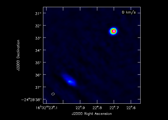
In Figure X we show the final image of all this process. The rms noise measured is XXX, the secondary beam resulted in XX XX PA. The peak values for the two components are XX and YY, while its fluxes are XX and YY. | In Figure X we show the final image of all this process. The rms noise measured is XXX, the secondary beam resulted in XX XX PA. The peak values for the two components are XX and YY, while its fluxes are XX and YY. | ||
[[File: | [[File:IRAS16293B9_contimage.png|200px|thumb|right|'''Fig. X.''' Continuum image resulted from the complete process of self calibration for the mosaic of IRAS16293 Band 9.]] | ||
Revision as of 21:24, 23 May 2012
Overview
This section of the casa guide continues from the last step of the calibration one. If you completed the calibration section, then you already have the final calibrated dataset. If you just started to work on this IRAS16293 B9 data, you can download the fully calibrated dataset IRAS16293_Band9_CalibratedMS from
This casa guide covers imaging of both continuum and line of IRAS16293 Band 9. The commands in this guide should be executed in CASA 3.4.0 since CASA 3.3.0 would be very slow for the cleaning process of a big dataset like this one for IRAS16293 Band 9. In this casa guide you will also need the Analysis Utils package, so make sure you have it imported into CASA.
Before we start with the imaging itself, do a listobs to the calibrated dataset, so you can check that everything is ok.
# listobs to check data
listobs(vis='IRAS16293_Band9.ms',
        listfile='IRAS16293_Band9.ms.listobs',verbose=F)
You should see the next information in the .listobs file.
Fields: 7
  ID   Code Name                RA              Decl          Epoch   SrcId
  0    none IRAS16293-2422-a    16:32:22.99200 -24.28.36.0000 J2000   0
  1    none IRAS16293-2422-a    16:32:22.47925 -24.28.36.0000 J2000   0
  2    none IRAS16293-2422-a    16:32:22.73563 -24.28.36.0000 J2000   0
  3    none IRAS16293-2422-a    16:32:22.73563 -24.28.32.5000 J2000   0
  4    none IRAS16293-2422-a    16:32:22.47925 -24.28.29.0000 J2000   0
  5    none IRAS16293-2422-a    16:32:22.73563 -24.28.29.0000 J2000   0
  6    none IRAS16293-2422-a    16:32:22.99200 -24.28.29.0000 J2000   0
   (nVis = Total number of time/baseline visibilities per field)
Spectral Windows:  (4 unique spectral windows and 1 unique polarization setups)
  SpwID  #Chans Frame Ch1(MHz)    ChanWid(kHz)  TotBW(kHz)  Corrs
  0        3840 TOPO  703312.744  488.28125     1875000     XX  YY
  1        3840 TOPO  692237.256  488.28125     1875000     XX  YY
  2        3840 TOPO  690437.256  488.28125     1875000     XX  YY
  3        3840 TOPO  688437.256  488.28125     1875000     XX  YY
Antennas: 14 'name'='station'
   ID=   0-3: 'DA41'='A003', 'DA43'='A075', 'DA47'='A026', 'DV02'='A077',
   ID=   4-7: 'DV03'='A137', 'DV05'='A082', 'DV07'='A076', 'DV09'='A046',
   ID=  8-11: 'DV10'='A071', 'DV12'='A011', 'DV13'='A072', 'DV14'='A025',
   ID= 12-13: 'DV17'='A138'
Continuum Emission Imaging
As it is shown in Figures 2 and 3 of IRAS16293Band9, these observations have a 7 pointing mosaic, which you can visualize with the next command (see also Figure 1).
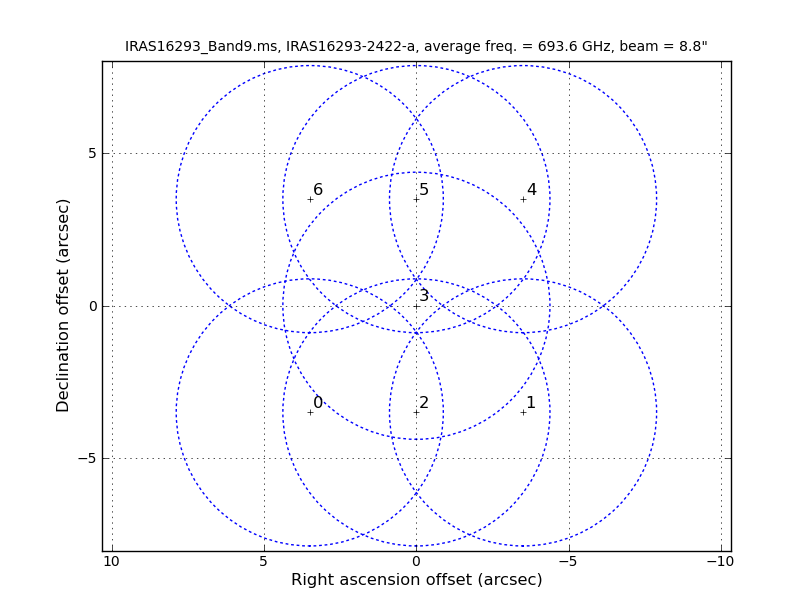
# Make a plot of the mosaic pattern with field ids identified
aU.plotMosaic(vis='IRAS16293_Band9.ms',sourceid='0',
              doplot=True,figfile='mosaic_pattern.png')
You might wander what of these pointings or fields have stronger line emission. You can know this by running the next command. We set spw='1' containing CO (6-5), and you can check all the plots for all the fields by just hitting the arrow for "next". Also see Figure 2 for an example of the output.
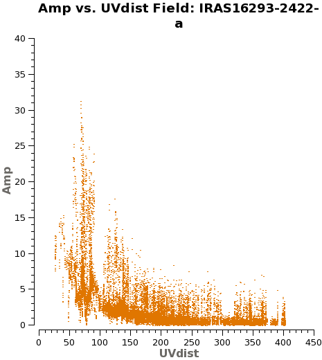
# See which mosaic fields have the brightest line emission
plotms(vis='IRAS16293_Band9.ms',
       field='',xaxis='uvdist', yaxis='amp',
       spw='1', avgchannel='3840',coloraxis='field',
       iteraxis='field')
Another way to visualize the uv-amp distribution is with the next plotms. This will load all the fields or pointing into the plot, and you can change interactively between the spws using the appropriate button in plotms. See Figure 3 for a plot of spw 1.
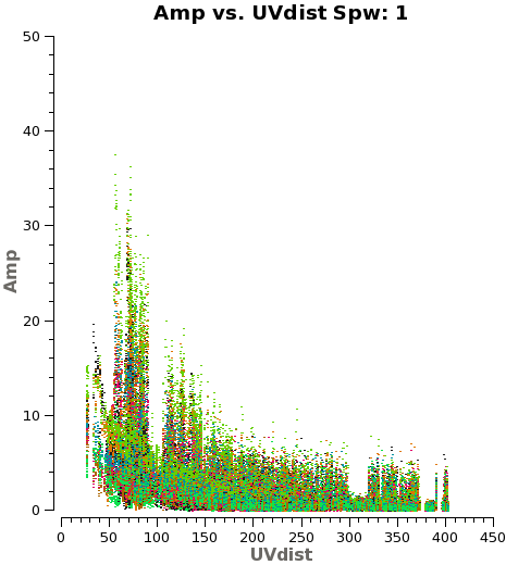
# Iterate over spws all fields
plotms(vis='IRAS16293_Band9.ms',
       field='',xaxis='uvdist', yaxis='amp',
       spw='', avgchannel='3840',coloraxis='field',
       iteraxis='spw')
We need to note the channels that do not present line emission. To identify them we can plot the amplitude vs frequency for all the spectral windows. Figure 4 shows the output from the next command for spw 1.
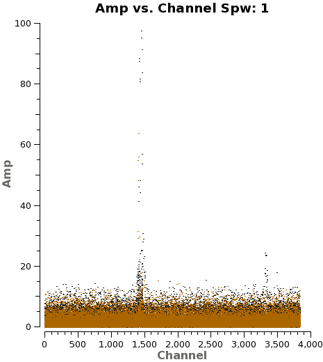
# Select Channels for uvcontsub. Average every 8 channels for
# increased S/N.

plotms(vis='IRAS16293_Band9.ms',
       xaxis='channel', yaxis='amp',field='0,4',
       spw='', avgtime='1e8',avgscan=T,coloraxis='field',
       avgchannel='8',iteraxis='spw',ydatacolumn='corrected',
       xselfscale=True,yselfscale=True)
Using the plots from the previous command you can select the line emission free channels just by looking for strong lines. To do this in the rigorous way, you would need to make dirty images and then select the continuum channels. Here we provide you with the channel selection we used for continuum emission.
Now uvcontsub will be used to calculate the level of continuum (based on your selection of continuum channels) and subtract that from the dataset.
# subtracting the continuum
contspw='0:20~1700;2500~3820,1:20~400;500~1100;1900~3000;3450~3800,2:20~1700;2200~3100,3:800~1600;2900~3300'
uvcontsub(vis='IRAS16293_Band9.ms',fitspw=contspw,fitorder=1,combine='spw')
The next flagmanager command will save the flags state in case you might need to re-do the continuum subtraction.
flagmanager(vis='IRAS16293_Band9.ms',mode='save',versionname='Original')

# NOTE: If uvcontsub needs to be run again restore flagged channels
# first
# flagmanager(vis='IRAS16293_Band9.ms',mode='restore',versionname='Original')
Now we will flag the channels we did not choose for continuum subtraction, ie the line emission channels. We will be left with only continuum channels.
# flagging the line channels
flagdata(vis='IRAS16293_Band9.ms',
         spw='0:1700~2500,1:400~500;1100~1900;3000~3450,2:1700~2200;3100~3840,3:0~800;1600~2900;3300~3840',flagbackup=F)
Note that more continuum imaging we do not need to have a high spectral resolution, so we will average 200 channels. This will help CASA imaging to run faster.
# Make a channel averaged version for speedier continuum imaging
split(vis='IRAS16293_Band9.ms',
      outputvis='IRAS16293_Band9_CONT.msAVG',field='',
      datacolumn='data',width=200,spw='0~3:20~3819')
Next you need to execute the next commands to fix some issues in the HISTORY section of the data.
# Fix a bug with History table
tb.open('IRAS16293_Band9_CONT.msAVG/HISTORY', nomodify = False)
a = tb.rownumbers()
tb.removerows(a)
tb.close()

tb.open('IRAS16293_Band9.ms.contsub/HISTORY', nomodify = False)
a = tb.rownumbers()
tb.removerows(a)
tb.close()
Clean and self-cal the continuum
Now we proceed with the cleaning itself. For the clean task you will need to choose the right cell size, map size, etc. Below are the parameters that were used in this casaguide. Note that the command will be interactive and you will have to set the cleaning boxes.
# cleaning the continuum
os.system('rm -rf *CONTIN*')
clean(vis='IRAS16293_Band9_CONT.msAVG',
     imagename='IRAS16293_Band9.CONTIN',
     spw='0~3',field='',phasecenter='3',
     mode='mfs',imagermode='mosaic',
     imsize=500,cell='0.04arcsec',minpb=0.25,
     interactive=T,
     weighting='briggs',robust=0.5,
     niter=10000, threshold='0.3mJy')
It is important to check if all fields have some emission in the model data column, if not, or very weak you would want to exclude from gaincal below. Because the bright Source B is in all the sidelobes all fields, do have some model data components.
# checking the model data for all the fields
plotms(vis='IRAS16293_Band9_CONT.msAVG',
      xaxis='time', yaxis='amp',field='',iteration='field',
      spw='', avgchannel='4000',coloraxis='field',
      ydatacolumn='model',xselfscale=True,yselfscale=True)
Now we proceed with gaincal to perform self calibration (for phases) on the data. Even with minsnr=3.0 there will be failed solutions.
# get one scan per field
os.system('rm -rf cont_pcal1')
gaincal(vis='IRAS16293_Band9_CONT.msAVG',caltable='cont_pcal1',gaintype='T',
        refant='DV14',calmode='p',combine='',spw='',field='',
        solint='inf',minsnr=3.0,minblperant=4)
The solutions for five antennas are shown in Figure 6, and are produced with the next plotcal. Be sure to check all the antennas.
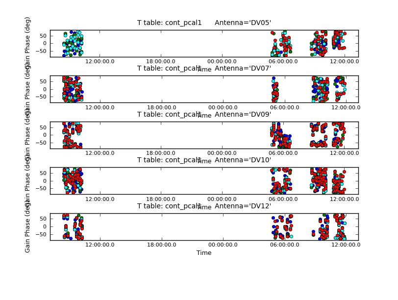
plotcal(caltable='cont_pcal1',xaxis='time',yaxis='phase',
        spw='',iteration='antenna',subplot=511,plotrange=[0,0,-80,80],
        antenna='',timerange='')

# The phases are remarkably stable for Band 9!
We then apply the table to the data to proceed right after with the proper cleaning, to check the improvement of the data.
# application of the table
applycal(vis='IRAS16293_Band9_CONT.msAVG',spwmap=[],spw='',
       gaintable=['cont_pcal1'],calwt=F,flagbackup=F)
Now you are ready for the second cleaning. For this one we are using the mask resulting from the previous cleaning. In the next blocks of commands we will repeat this process (clean, viewer, gaincal, plotcal, applycal, clean, etc) to improve the overall quality of the image.
# cleaning
os.system('rm -rf *CONTIN_P1*')
clean(vis='IRAS16293_Band9_CONT.msAVG',
     imagename='IRAS16293_Band9.CONTIN_P1',
     spw='0~3',field='',phasecenter='3',
     mode='mfs',imagermode='mosaic',
     imsize=500,cell='0.04arcsec',minpb=0.25,
     interactive=T,
     weighting='briggs',robust=0.5,
     mask='IRAS16293_Band9.CONTIN.mask',
     niter=10000, threshold='0.3mJy')

# visualize the image
imview (raster=[{'file':'IRAS16293_Band9.CONTIN.image',
                 'range': [-0.01,0.5]},
                {'file': 'IRAS16293_Band9.CONTIN_P1.image',
                 'range': [-0.01,0.5]}])
Second gaincal step for self calibration.
# second self-cal
os.system('rm -rf cont_pcal2')
gaincal(vis='IRAS16293_Band9_CONT.msAVG',caltable='cont_pcal2',gaintype='T',
        refant='DV14',calmode='p',combine='',spw='',field='',
        solint='inf',minsnr=3.0,minblperant=4)

#Checking the table
plotcal(caltable='cont_pcal2',xaxis='time',yaxis='phase',
        spw='',iteration='antenna',subplot=511,plotrange=[0,0,-80,80],
        antenna='',timerange='')

# Applying results to the data
applycal(vis='IRAS16293_Band9_CONT.msAVG',spwmap=[],spw='',
       gaintable=['cont_pcal2'],calwt=F,flagbackup=F)
We continue with the next cleaning.
os.system('rm -rf *CONTIN_P2*')
clean(vis='IRAS16293_Band9_CONT.msAVG',
     imagename='IRAS16293_Band9.CONTIN_P2',
     spw='0~3',field='',phasecenter='3',
     mode='mfs',imagermode='mosaic',
     imsize=500,cell='0.04arcsec',minpb=0.25,
     interactive=T,
     weighting='briggs',robust=0.5,
     mask='IRAS16293_Band9.CONTIN.mask',
     niter=10000, threshold='0.3mJy')

# to view the resulting image
imview (raster=[{'file':'IRAS16293_Band9.CONTIN_P1.image',
                 'range': [-0.01,0.5]},
                {'file': 'IRAS16293_Band9.CONTIN_P2.image',
                 'range': [-0.01,0.5]}])

# There is very little change, the bold could try another iteration using a shorter
# solint phase self-cal. For now, moving on to amplitude.
Next iteration with gaincal, now using amplitude and phase for "calmode".
# For amplitude self-cal we only want to get one solution per spw, per dataset
os.system('rm -rf cont_apcal')
gaincal(vis='IRAS16293_Band9_CONT.msAVG',caltable='cont_apcal',gaintype='T',
        refant='DV14',calmode='ap',combine='scan,field',spw='',field='',
        solint='8000s',minsnr=3.0,minblperant=4,gaintable='cont_pcal2')

# ploting the table
plotcal(caltable='cont_apcal',xaxis='time',yaxis='amp',
        spw='',iteration='antenna',subplot=511,plotrange=[0,0,0.5,2],
        antenna='',timerange='')

# and applying to the data
applycal(vis='IRAS16293_Band9_CONT.msAVG',spwmap=[],spw='',
       gaintable=['cont_pcal2','cont_apcal'],calwt=F,flagbackup=F)

# A large correction is present for the 2nd dataset. This amplitude
# error was causing many of the artifacts noticeable in the previous
# images.
Continuing the the proper cleaning step.
# new cleaning for self-cal using calmode='ap'
os.system('rm -rf *CONTIN_AP*')
clean(vis='IRAS16293_Band9_CONT.msAVG',
     imagename='IRAS16293_Band9.CONTIN_AP',
     spw='0~3',field='',phasecenter='3',
     mode='mfs',imagermode='mosaic',
     imsize=500,cell='0.04arcsec',minpb=0.25,
     interactive=T,
     weighting='briggs',robust=0.5,
     mask='IRAS16293_Band9.CONTIN_P2.mask',
     niter=10000, threshold='0.3mJy')

# and to view the image
imview (raster=[{'file':'IRAS16293_Band9.CONTIN_P2.image',
                 'range': [-0.01,0.5]},
                {'file': 'IRAS16293_Band9.CONTIN_AP.image',
                 'range': [-0.01,0.5]}])
We use now impbcor to produce an image corrected by the primary beam.
# correting for primary beam
impbcor(imagename='IRAS16293_Band9.CONTIN_AP.image',
        pbimage='IRAS16293_Band9.CONTIN_AP.flux',
        outfile='IRAS16293_Band9.CONTIN_AP.image.pbcor.subim',
        box='120,104,315,299')

# and checking the image
imview (raster=[{'file':'IRAS16293_Band9.CONTIN_AP.image',
                 'range': [-0.01,0.5]},
                {'file': 'IRAS16293_Band9.CONTIN_AP.image.pbcor',
                 'range': [-0.01,0.5]}])
In Figure X we show the final image of all this process. The rms noise measured is XXX, the secondary beam resulted in XX XX PA. The peak values for the two components are XX and YY, while its fluxes are XX and YY.
Now you can export your final image in fits format, so you can analyze it anytime.
exportfits(imagename='IRAS16293_Band9.CONTIN_AP.image.pbcor.subim',
           fitsimage='IRAS16293_Band9.CONTIN_AP.image.pbcor.subim.fits')
Last checked on CASA Version 3.4.0.