IRAS16293 Band9 - Calibration for CASA 3.3: Difference between revisions
No edit summary |
No edit summary |
||
| Line 785: | Line 785: | ||
In Figure 5 we show an output example for this command. | In Figure 5 we show an output example for this command. | ||
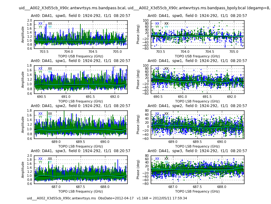
[[File:uid___A002_X3d55cb_X90c.antwvrtsys.ms.bandpass_bpoly.DA41.spw0.t1|200px|thumb|right|'''Fig. 5.''' Bandpass solutions for the dataset X90c showing antenna DA41. Both amplitude and phases solutions are plotted.]] | [[File:uid___A002_X3d55cb_X90c.antwvrtsys.ms.bandpass_bpoly.DA41.spw0.t1.png|200px|thumb|right|'''Fig. 5.''' Bandpass solutions for the dataset X90c showing antenna DA41. Both amplitude and phases solutions are plotted.]] | ||
Revision as of 15:53, 22 May 2012
- This script assumes that you have downloaded IRAS16293_Band9_UnCalibratedMSAndTablesForReduction.tgz from IRAS16293Band9#Download the data
- Details of the ALMA observations are provided at IRAS16293Band9
- This portion of the guide covers calibration of the raw visibility data. To skip to the imaging portion of the guide, see: IRAS16293_Band9_-_Imaging.
Overview
This part of the casa guide will guide you through the basic inspection of the data, paying special attention to detect data that needs to be flagged. The guide goes later to the process of full calibration to split the data at the end.
The general procedure in this guide follows the other ALMA CASA guides: NGC3256Band3 and AntennaeBand7.
Unpack the Data
Once you have downloaded the IRAS16293_Band9_UnCalibratedMSandTablesForReduction.tgz, unpack the file in a terminal outside CASA using
tar -xvzf IRAS16293_Band9_UnCalibratedMSandTablesForReduction.tgz

cd IRAS16293_Band9_UnCalibratedMSandTablesForReduction
You have a number of files with extensions ".ms", which are CASA measurement set (MS) files. You will also see files containing system temperature (Tsys), water vapor radiometer (WVR), and antenna position information.
To start CASA type
casapy
Be sure that you are using the right version indicated for this guide.
Initial Inspection
The first step we will do through all the calibration process is to define an array with the uid's that corresponds to the datasets names. This will allow to make the calibration of the four datasets one after another, using an for-loop inside python. We will then calibrate the data individually and concatenate them at the end, before proceeding with the imaging part.
Note that if you exit CASA and want to continue with the calibration using these arrays, you will have to re-issue the command again to make it available for the current CASA execution.
To start, and give an example of this process, we will create txt format files for the output of the listobs task, which will give us useful information about the observations.
# Array containing the names of the uids

rawdata=['uid___A002_X3d4118_X39b.ms','uid___A002_X3d55cb_X575.ms',
         'uid___A002_X3d55cb_Xb50.ms','uid___A002_X3d55cb_X90c.ms']

# We create the text files for listobs for each dataset

for data in rawdata:
  listobs(vis=data,listfile=data+'.listobs')
Note that after cutting and pasting a for-loop you often have to press return several times to make the command executes. The output will be sent to the CASA logger. Next there is an example of a useful part of the output that the first listobs of the previews command produces.
Fields: 11 ID Code Name RA Decl Epoch SrcId nVis 0 none 1924-292 19:24:51.05600 -29.14.30.1280 J2000 0 169125 1 none nrao530 ph 17:33:02.72400 -13.04.49.4860 J2000 1 289170 2 none Juno 16:25:31.63031 -05.49.08.9209 J2000 2 82890 3 none 1625-254 16:25:46.98000 -25.27.38.3300 J2000 3 276480 4 none IRAS16293-2422-a 16:32:22.99200 -24.28.36.0000 J2000 4 132450 5 none IRAS16293-2422-a 16:32:22.47925 -24.28.36.0000 J2000 4 99915 6 none IRAS16293-2422-a 16:32:22.73563 -24.28.36.0000 J2000 4 99960 7 none IRAS16293-2422-a 16:32:22.73563 -24.28.32.5000 J2000 4 99915 8 none IRAS16293-2422-a 16:32:22.47925 -24.28.29.0000 J2000 4 99945 9 none IRAS16293-2422-a 16:32:22.73563 -24.28.29.0000 J2000 4 99945 10 none IRAS16293-2422-a 16:32:22.99200 -24.28.29.0000 J2000 4 99915 (nVis = Total number of time/baseline visibilities per field) Spectral Windows: (25 unique spectral windows and 2 unique polarization setups) SpwID #Chans Frame Ch1(MHz) ChanWid(kHz) TotBW(kHz) Corrs 0 4 TOPO 184550 1500000 7500000 I 1 128 TOPO 231257.813 15625 2000000 XX YY 2 1 TOPO 232234.375 1796875 1796875 XX YY 3 128 TOPO 229257.813 15625 2000000 XX YY 4 1 TOPO 230234.375 1796875 1796875 XX YY 5 128 TOPO 217242.188 15625 2000000 XX YY 6 1 TOPO 216234.375 1796875 1796875 XX YY 7 128 TOPO 215242.188 15625 2000000 XX YY 8 1 TOPO 214234.375 1796875 1796875 XX YY 9 128 TOPO 703257.813 15625 2000000 XX YY 10 1 TOPO 704234.375 1796875 1796875 XX YY 11 128 TOPO 692492.188 15625 2000000 XX YY 12 1 TOPO 691484.375 1796875 1796875 XX YY 13 128 TOPO 690492.188 15625 2000000 XX YY 14 1 TOPO 689484.375 1796875 1796875 XX YY 15 128 TOPO 688492.188 15625 2000000 XX YY 16 1 TOPO 687484.375 1796875 1796875 XX YY 17 3840 TOPO 703312.744 488.28125 1875000 XX YY 18 1 TOPO 704249.756 1875000 1875000 XX YY 19 3840 TOPO 692237.256 488.28125 1875000 XX YY 20 1 TOPO 691299.756 1875000 1875000 XX YY 21 3840 TOPO 690437.256 488.28125 1875000 XX YY 22 1 TOPO 689499.756 1875000 1875000 XX YY 23 3840 TOPO 688437.256 488.28125 1875000 XX YY 24 1 TOPO 687499.756 1875000 1875000 XX YY Sources: 176 ID Name SpwId RestFreq(MHz) SysVel(km/s) 0 1924-292 0 - - 0 1924-292 25 - - 0 1924-292 26 - - 0 1924-292 27 - - 0 1924-292 28 - - 0 1924-292 29 - - 0 1924-292 30 - - 0 1924-292 31 - - 0 1924-292 32 - - 0 1924-292 33 - - 0 1924-292 34 - - 0 1924-292 35 - - 0 1924-292 36 - - 0 1924-292 37 - - 0 1924-292 38 - - 0 1924-292 39 - - 0 1924-292 1 - - 0 1924-292 2 - - 0 1924-292 3 - - 0 1924-292 4 - - 0 1924-292 5 - - 0 1924-292 6 - - 0 1924-292 7 - - 0 1924-292 8 - - 0 1924-292 9 - - 0 1924-292 10 - - 0 1924-292 11 - - 0 1924-292 12 - - 0 1924-292 13 - - 0 1924-292 14 - - 0 1924-292 15 - - 0 1924-292 16 - - 0 1924-292 17 - - 0 1924-292 18 - - 0 1924-292 19 - - 0 1924-292 20 - - 0 1924-292 21 - - 0 1924-292 22 - - 0 1924-292 23 - - 0 1924-292 24 - - 1 nrao530 ph 0 - - 1 nrao530 ph 25 - - 1 nrao530 ph 26 - - 1 nrao530 ph 27 - - 1 nrao530 ph 28 - - 1 nrao530 ph 29 - - 1 nrao530 ph 30 - - 1 nrao530 ph 31 - - 1 nrao530 ph 32 - - 1 nrao530 ph 33 - - 1 nrao530 ph 34 - - 1 nrao530 ph 35 - - 1 nrao530 ph 36 - - 1 nrao530 ph 37 - - 1 nrao530 ph 38 - - 1 nrao530 ph 39 - - 1 nrao530 ph 1 - - 1 nrao530 ph 2 - - 1 nrao530 ph 3 - - 1 nrao530 ph 4 - - 1 nrao530 ph 5 - - 1 nrao530 ph 6 - - 1 nrao530 ph 7 - - 1 nrao530 ph 8 - - 2 Juno 0 - - 2 Juno 25 - - 2 Juno 26 - - 2 Juno 27 - - 2 Juno 28 - - 2 Juno 29 - - 2 Juno 30 - - 2 Juno 31 - - 2 Juno 32 - - 2 Juno 33 - - 2 Juno 34 - - 2 Juno 35 - - 2 Juno 36 - - 2 Juno 37 - - 2 Juno 38 - - 2 Juno 39 - - 1 Juno 9 - - 1 Juno 10 - - 1 Juno 11 - - 1 Juno 12 - - 1 Juno 13 - - 1 Juno 14 - - 1 Juno 15 - - 1 Juno 16 - - 1 Juno 17 - - 1 Juno 18 - - 1 Juno 19 - - 1 Juno 20 - - 1 Juno 21 - - 1 Juno 22 - - 1 Juno 23 - - 1 Juno 24 - - 3 1625-254 0 - - 3 1625-254 25 - - 3 1625-254 26 - - 3 1625-254 27 - - 3 1625-254 28 - - 3 1625-254 29 - - 3 1625-254 30 - - 3 1625-254 31 - - 3 1625-254 32 - - 3 1625-254 33 - - 3 1625-254 34 - - 3 1625-254 35 - - 3 1625-254 36 - - 3 1625-254 37 - - 3 1625-254 38 - - 3 1625-254 39 - - 2 1625-254 1 - - 2 1625-254 2 - - 2 1625-254 3 - - 2 1625-254 4 - - 2 1625-254 5 - - 2 1625-254 6 - - 2 1625-254 7 - - 2 1625-254 8 - - 2 1625-254 17 - - 2 1625-254 18 - - 2 1625-254 19 - - 2 1625-254 20 - - 2 1625-254 21 - - 2 1625-254 22 - - 2 1625-254 23 - - 2 1625-254 24 - - 2 nrao530 ph 9 - - 2 nrao530 ph 10 - - 2 nrao530 ph 11 - - 2 nrao530 ph 12 - - 2 nrao530 ph 13 - - 2 nrao530 ph 14 - - 2 nrao530 ph 15 - - 2 nrao530 ph 16 - - 3 nrao530 ph 17 - - 3 nrao530 ph 18 - - 3 nrao530 ph 19 - - 3 nrao530 ph 20 - - 3 nrao530 ph 21 - - 3 nrao530 ph 22 - - 3 nrao530 ph 23 - - 3 nrao530 ph 24 - - 4 IRAS16293-2422-a 0 - - 4 IRAS16293-2422-a 25 - - 4 IRAS16293-2422-a 26 - - 4 IRAS16293-2422-a 27 - - 4 IRAS16293-2422-a 28 - - 4 IRAS16293-2422-a 29 - - 4 IRAS16293-2422-a 30 - - 4 IRAS16293-2422-a 31 - - 4 IRAS16293-2422-a 32 - - 4 IRAS16293-2422-a 33 - - 4 IRAS16293-2422-a 34 - - 4 IRAS16293-2422-a 35 - - 4 IRAS16293-2422-a 36 - - 4 IRAS16293-2422-a 37 - - 4 IRAS16293-2422-a 38 - - 4 IRAS16293-2422-a 39 - - 3 IRAS16293-2422-a 9 - - 3 IRAS16293-2422-a 10 - - 3 IRAS16293-2422-a 11 - - 3 IRAS16293-2422-a 12 - - 3 IRAS16293-2422-a 13 - - 3 IRAS16293-2422-a 14 - - 3 IRAS16293-2422-a 15 - - 3 IRAS16293-2422-a 16 - - 4 IRAS16293-2422-a 17 - - 4 IRAS16293-2422-a 18 - - 4 IRAS16293-2422-a 19 - - 4 IRAS16293-2422-a 20 - - 4 IRAS16293-2422-a 21 - - 4 IRAS16293-2422-a 22 - - 4 IRAS16293-2422-a 23 - - 4 IRAS16293-2422-a 24 - - Antennas: 15: ID Name Station Diam. Long. Lat. 0 DA41 A003 12.0 m -067.45.16.5 -22.53.27.0 1 DA43 A075 12.0 m -067.45.17.9 -22.53.21.4 2 DA47 A026 12.0 m -067.45.18.8 -22.53.28.3 3 DV02 A077 12.0 m -067.45.10.1 -22.53.25.9 4 DV03 A137 12.0 m -067.45.15.2 -22.53.22.7 5 DV05 A082 12.0 m -067.45.08.3 -22.53.29.2 6 DV07 A076 12.0 m -067.45.20.5 -22.53.33.8 7 DV09 A046 12.0 m -067.45.17.0 -22.53.29.3 8 DV10 A071 12.0 m -067.45.19.9 -22.53.23.5 9 DV12 A011 12.0 m -067.45.14.4 -22.53.28.4 10 DV13 A072 12.0 m -067.45.12.6 -22.53.24.0 11 DV14 A025 12.0 m -067.45.18.7 -22.53.27.4 12 DV15 A074 12.0 m -067.45.12.1 -22.53.32.0 13 DV17 A138 12.0 m -067.45.17.1 -22.53.34.4 14 DV18 A053 12.0 m -067.45.17.3 -22.53.31.2
You can see the ID that is assigned for each source, starting with ID 0. 1924-292 and 3c279 are the calibrators for bandpass, Juno for amplitud (flux), 1625-254 and nrao530 ph are for phase calibration, and the remaining 7 fields of IRAS16293-2422-a are the seven pointings for our mosaic of the target source.
Spectral windows are also marked with numbers from 0 24, with 0 containing WVR information. Spws 17, 19, 21, and 23 contain the sience data (TDM mode). The CO (6-5) line emission is contained in spw 21. Spw 18, 20, 22, and 24 contain channel averages of the data in spectral windows 17, 19, 21, 23, respectively. These spws will not be used for the offline data reduction. All the remaining spw that appear in the section of sources, and that do not appear in the Spectral Windows are related to WVR measurements for each antenna, so you will not need them for the calibration. Spws 9, 11, 13, and 15 are associated with tsys measurements, and we will apply these information to the science spws later.
Visualization and application of Tsys and WVR tables
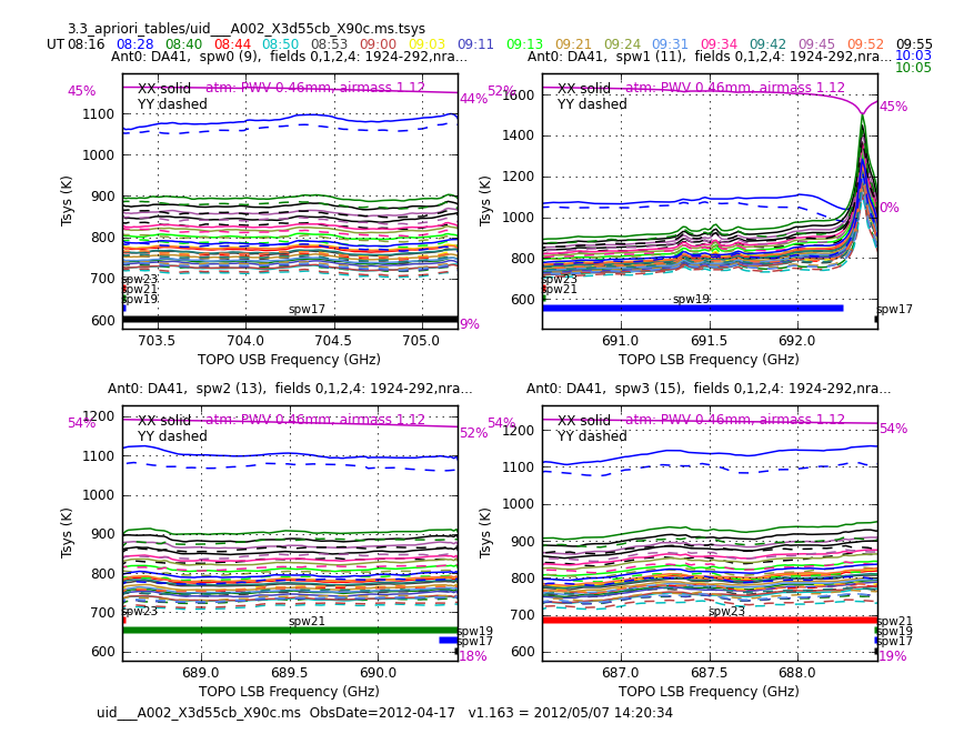
Next we need to check the plotting for tsys and wvr tables to make sure whether they have issues that might affect their application to the data. Whenever we see an odd behavior in the tables we need to flag the corresponding sience data to prevent wrong results in the calibration steps. The next command, that comes from the Analysis Utils package will plot the tsys in the next way: it will produce many plots, each one of them will show an antenna, with the four spw that tsys covers, for all the targets, and with different colors for different times, so you can trace the behavior for tsys with time, among others. Note that in spw 19 and 21, the overlap with the tsys spw (11 and 13) is not set correctly. This is due to an error in the frequencies for the tsys when the observations were done. You do not have to worry about this, since any issue coming from the error have already been handled. Note, however that the portions of the spectra that do not have tsys information cannot be used. This does not represent a problem, since that part corresponds to the edge of the baseband. Also note that the CO (6-5) line is not affected by this. In Figure 1 you will see the corresponding plot for one of the datasets (X90c) showing antenna 0 (DA41).
# Plot TDM Tsys tables, and show locations of FDM spws
os.system('rm -rf Tsysplots')
for vis in rawdata:
  aU.plotbandpass('3.3_apriori_tables/'+vis+'.tsys',ms=vis,
                overlay='time', xaxis='freq',
                yaxis='amp',subplot=22,interactive=False,
                showatm=True,
                chanrange='5~122',showfdm=True,
                figfile='Tsysplots/'+vis+'tsys.png')
Make sure that you notice all the next issues with tsys, since we will need to flag the corresponding science data.
 X90c
 DV05 ripples all spw
 Otherwise 600 to 1200 47 to 57% transmission

 X575
 Otherwise 1300 to 3000 28 to 39% transmission
 DV05 ripples all spw

 Xb50
 800 to 2500 37 to 47% transmission
 DV05 ripples all spw

 X39b
 500 to 800 56 to 65%
 DA43 Tsys crazy for spw=23
 DV05 ripples all spw and one time with bad YY
 DV18 crazy for spw=23
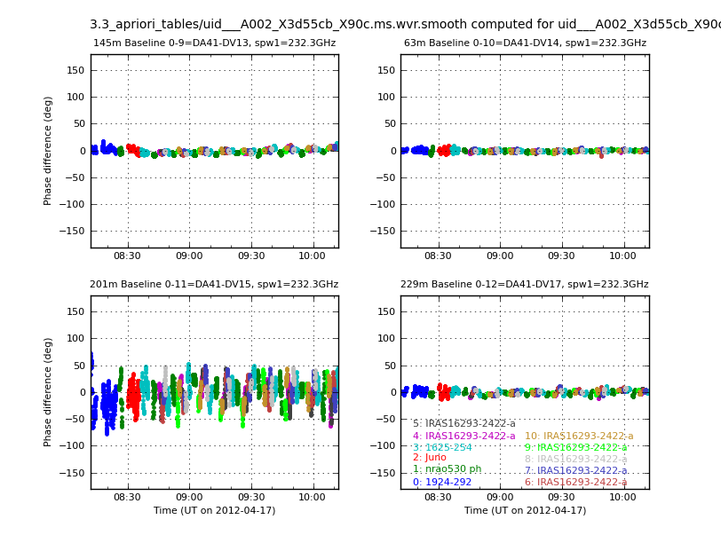
Now, for the plotting of the wvr tables, we will employ again the analysis utils. This commands will create a directory with many plots inside, each one of them corresponding to different datasets, baselines and targets, using different colors. In Figure 2 you can see an example of the output for spectral window 1. Note that the command below only creates the tables for that spw, since the others are the same except for a scale factor that is the ratio of frequencies.
Note that in all datasets, DV15 has bad wvr behavior.
# Plotting wvr tables for spw 1
os.system('rm -rf WVRplots')
for vis in rawdata:
  aU.plotWVRSolutions(caltable='3.3_apriori_tables/'+vis+'.wvr.smooth',
              yrange=[-180,180],figfile='WVRplots/'+vis+'.wvr.smooth.png',
              ms=vis,spw='1',interactive=False)
Before you continue it is important you save the flags status, so you can recover this state if you need it while redoing the calibration.
rawdata=['uid___A002_X3d4118_X39b.ms','uid___A002_X3d55cb_X575.ms',
         'uid___A002_X3d55cb_Xb50.ms','uid___A002_X3d55cb_X90c.ms']

for vis in rawdata:
  flagmanager(vis=vis,mode='save',versionname='Original')
Now, based on the behavior of the tsys and wvr tables, we will flag the corresponding data. The next commands will do so. You can employ similar executions to flag other data you might want to remove.
# Flagging corresponding science data for tsys and wvr showing problems
for vis in rawdata:
  flagdata(vis=vis,autocorr = T,flagbackup = F)
  flagdata(vis=vis,mode='shadow',flagbackup=F)
  flagdata(vis=vis,antenna='DV15',flagbackup=F)

vis='uid___A002_X3d4118_X39b.ms'
flagdata(vis=vis,antenna='DA43,DV18',spw='23',flagbackup=F)

# For now leave DV05 in but keep an eye on it.
Applying tsys and wvr tables and splitting the data
As you could see from the initial application of listobs, 1924-292 is the bandpass calibrator for three of the datasets, and 3c279 is for one of them. For this reason, the application of the tables is split in two parts. Ignore the warnings from the first application execution of applycal, since it does not harm the data.
# Re-entering our array

rawdata=['uid___A002_X3d4118_X39b.ms','uid___A002_X3d55cb_X575.ms',
         'uid___A002_X3d55cb_Xb50.ms','uid___A002_X3d55cb_X90c.ms']

# Separate sources with Tsys measurements of their own from those that
# do not. Since only one IRAS16293 field (id=4) has Tsys, it goes into the
# "not" category.

field_Tsys=['1924-292','nrao530 ph','Juno']
field_noTsys=['1625-254','IRAS16293*']

for vis in rawdata:
  for field in field_Tsys:
    applycal(vis=vis,field=field,
             spw = '17,19,21,23',
             gaintable = ['3.3_apriori_tables/'+vis+'.tsys.fdm',
                          '3.3_apriori_tables/'+vis+'.wvr.smooth',
                          '3.3_apriori_tables/'+vis+'.antpos'],
             gainfield = [field,field,''],
             interp = ['linear','nearest',''],calwt = T,
             flagbackup = F)

# This one dataset has 3C279 instead of 1924-292 as the bpcal and is the
# source of warnings in prevoius applycal

vis='uid___A002_X3d55cb_X575.ms'
field='3c279'
applycal(vis=vis,field=field,
             spw = '17,19,21,23',
             gaintable = ['3.3_apriori_tables/'+vis+'.tsys.fdm',
                          '3.3_apriori_tables/'+vis+'.wvr.smooth',
                          '3.3_apriori_tables/'+vis+'.antpos'],
             gainfield = [field,field,''],
             interp = ['linear','nearest',''],calwt = T,
             flagbackup = F)

for vis in rawdata:
  for field in field_noTsys:
    applycal(vis =vis,field=field,
             spw = '17,19,21,23',
             gaintable = ['3.3_apriori_tables/'+vis+'.tsys.fdm',
                          '3.3_apriori_tables/'+vis+'.wvr.smooth',
                          '3.3_apriori_tables/'+vis+'.antpos'],
             gainfield = ['4',field,''],
             interp = ['linear','nearest',''],calwt = T,
             flagbackup = F)

# Splitting the science spws

sciencespw='17,19,21,23'
for vis in rawdata:
  split(vis=vis,outputvis=('%s.antwvrtsys.ms'%(vis.split('.')[0])),datacolumn='corrected',spw=sciencespw,keepflags=False)
Data inspection
We now need to check any bad behavior in the data through several plots. Once problems are identified, corresponding data can be flagged. But before that, we need to run again listobs to check that the split worked as expected. We will define our array of new split datasets, along with a list of intents that will be useful in the next steps.
# New array of datasets
data=['uid___A002_X3d4118_X39b.antwvrtsys.ms',
      'uid___A002_X3d55cb_X575.antwvrtsys.ms',
      'uid___A002_X3d55cb_X90c.antwvrtsys.ms',
      'uid___A002_X3d55cb_Xb50.antwvrtsys.ms']

# Match up intents with source names
pcal='1625-254'
fluxcal='Juno'
science='IRAS16293*'
check='nrao530*'
bpcal=['1924-292','3c279','1924-292','1924-292']
calfields=['1924-292,Juno,1625-254,nrao530*',
           '3c279,Juno,1625-254,nrao530*',
           '1924-292,Juno,1625-254,nrao530*',
           '1924-292,Juno,1625-254,nrao530*']

for vis in data:
    listobs(vis=vis,listfile=vis+'.listobs',verbose=True)
You can explore any of the output files by doing cat file.listobs or using any other text viewer from a terminal not running CASA. Next you can see the output for X90c, and you will see the change in the spw naming, among others.
Fields: 11
  ID   Code Name                RA              Decl          Epoch   SrcId nVis
  0    none 1924-292            19:24:51.05600 -29.14.30.1280 J2000   0     13200
  1    none nrao530 ph          17:33:02.72400 -13.04.49.4860 J2000   1     23760
  2    none Juno                16:25:05.61170 -05.43.27.9210 J2000   2     10560
  3    none 1625-254            16:25:46.98000 -25.27.38.3300 J2000   3     26400
  4    none IRAS16293-2422-a    16:32:22.99200 -24.28.36.0000 J2000   4     11880
  5    none IRAS16293-2422-a    16:32:22.47925 -24.28.36.0000 J2000   4     11880
  6    none IRAS16293-2422-a    16:32:22.73563 -24.28.36.0000 J2000   4     11880
  7    none IRAS16293-2422-a    16:32:22.73563 -24.28.32.5000 J2000   4     11880
  8    none IRAS16293-2422-a    16:32:22.47925 -24.28.29.0000 J2000   4     10560
  9    none IRAS16293-2422-a    16:32:22.73563 -24.28.29.0000 J2000   4     10560
  10   none IRAS16293-2422-a    16:32:22.99200 -24.28.29.0000 J2000   4     10560
   (nVis = Total number of time/baseline visibilities per field)
Spectral Windows:  (4 unique spectral windows and 1 unique polarization setups)
  SpwID  #Chans Frame Ch1(MHz)    ChanWid(kHz)  TotBW(kHz)  Corrs
  0        3840 TOPO  703312.744  488.28125     1875000     XX  YY
  1        3840 TOPO  692237.256  488.28125     1875000     XX  YY
  2        3840 TOPO  690437.256  488.28125     1875000     XX  YY
  3        3840 TOPO  688437.256  488.28125     1875000     XX  YY
Sources: 20
  ID   Name                SpwId RestFreq(MHz)  SysVel(km/s)
  0    1924-292            0     -              -
  0    1924-292            1     -              -
  0    1924-292            2     -              -
  0    1924-292            3     -              -
  1    Juno                0     -              -
  1    Juno                1     -              -
  1    Juno                2     -              -
  1    Juno                3     -              -
  2    1625-254            0     -              -
  2    1625-254            1     -              -
  2    1625-254            2     -              -
  2    1625-254            3     -              -
  3    nrao530 ph          0     -              -
  3    nrao530 ph          1     -              -
  3    nrao530 ph          2     -              -
  3    nrao530 ph          3     -              -
  4    IRAS16293-2422-a    0     -              -
  4    IRAS16293-2422-a    1     -              -
  4    IRAS16293-2422-a    2     -              -
  4    IRAS16293-2422-a    3     -              -
Antennas: 12:
  ID   Name  Station   Diam.    Long.         Lat.
  0    DA41  A003      12.0 m   -067.45.16.5  -22.53.27.0
  1    DA43  A075      12.0 m   -067.45.17.9  -22.53.21.4
  2    DV02  A077      12.0 m   -067.45.10.1  -22.53.25.9
  3    DV03  A137      12.0 m   -067.45.15.2  -22.53.22.7
  4    DV05  A082      12.0 m   -067.45.08.3  -22.53.29.2
  5    DV07  A076      12.0 m   -067.45.20.5  -22.53.33.8
  6    DV09  A046      12.0 m   -067.45.17.0  -22.53.29.3
  7    DV10  A071      12.0 m   -067.45.19.9  -22.53.23.5
  8    DV12  A011      12.0 m   -067.45.14.4  -22.53.28.4
  9    DV13  A072      12.0 m   -067.45.12.6  -22.53.24.0
  10   DV14  A025      12.0 m   -067.45.18.7  -22.53.27.4
  12   DV17  A138      12.0 m   -067.45.17.1  -22.53.34.4
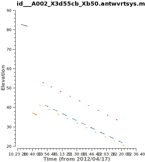
As we noted before, these observations contain datasets that were taken before and after transit of the science target. Elevation is especially important at Band 9 due to the increased airmass at low elevation and corresponding drop in transmission. By making plots for this we will note which datasets might be more affected by low elevation. In Figure 3 you can see the output of this command for Xb50.
# Elevation plots to understand what the elevation range for each dataset is.
for vis in data:
  plotms(vis=vis,
       field='',xaxis='time', yaxis='elevation',antenna='',
       spw='0', avgchannel='3840',coloraxis='field',
       ydatacolumn='data',plotfile=vis+'elevation.png',title=vis)
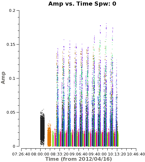
Next, we give you a set of useful plotms commands which will help you to analyze all the data in several ways. You can save a copy of the output, so you do not have to run them again every time you want to check them. This is especially useful for the ones that take a lot of time to complete. In Figure 4 you can see the output of the following plotms command. By clicking the "Next" arrow in plotms you can access the remaining spws, since the command was executed with the option iteraxis='spw'.
# Check overall behavior with time
vis=data[0]
plotms(vis=vis,
       field='',xaxis='time', yaxis='amp',antenna='',
       spw='', avgchannel='3840',coloraxis='field',
       iteraxis='spw',ydatacolumn='data',yselfscale=True)
For the next plotms commands, inspect each dataset, noting any problems that you notice.
# For at least one spw go antenna by antenna to look for dropouts not
# obvious in previous plot
vis=data[0]
plotms(vis=vis,
       field='',xaxis='time', yaxis='amp',antenna='',
       spw='2', avgchannel='3840',coloraxis='field',
       iteraxis='antenna',ydatacolumn='data')

# Check out spectral properties of each source for problems
vis=data[0]
plotms(vis=vis,
       field='',xaxis='freq', yaxis='amp',antenna='',
       spw='', avgtime='1e8',avgscan=True,coloraxis='spw',
       iteraxis='field',ydatacolumn='data',yselfscale=True)

# Examine phase of the bandpass calibrator for any problems
vis=data[0]
bp=bpcal[0]
plotms(vis=vis,
       field=bp,xaxis='freq', yaxis='phase',antenna='',
       spw='', avgtime='1e8',avgscan=True,avgchannel='10',coloraxis='spw',
       iteraxis='baseline',ydatacolumn='data',yselfscale=True)
Flagging
Next, based on our inspection we will proceed with the corresponding flagging. But before that, we will save the current flags state, so we can recover it later, if needed.
data=['uid___A002_X3d4118_X39b.antwvrtsys.ms',
      'uid___A002_X3d55cb_X575.antwvrtsys.ms',
      'uid___A002_X3d55cb_X90c.antwvrtsys.ms',
      'uid___A002_X3d55cb_Xb50.antwvrtsys.ms']

# Back up flag state in case you want to start over.
for vis in data:
  flagmanager(vis=vis,mode='save',versionname='Original')

# If you do start over run this first
for vis in data:
  flagmanager(vis=vis,mode='restore',versionname='Original')
Next, we proceed to flag the bad data. Here is the list of flags that we will do. If you note some other data that needs to be flagged, proceed with that.
# DV07 low amp after certain time. DV17 also but not as bad.
flagdata(vis='uid___A002_X3d55cb_X575.antwvrtsys.ms',
         antenna='DV07', timerange='>05:20:00',flagbackup=F)
Now, during the procedure of calibration we noted some problems in the data. So, it was needed to flag those data, and do the calibration again. In order to save your time, we note here those problems, so you can flag the data now.
# AFTER INITIAL CALIBRATION INSPECTION

# flag low elevation scans on 1625-254 and IRAS16293
flagdata(vis='uid___A002_X3d55cb_Xb50.antwvrtsys.ms',
         timerange='>12:03:00', field='',flagbackup=F)

# flag low gains on DV02 on Juno
flagdata(vis='uid___A002_X3d55cb_Xb50.antwvrtsys.ms',
         antenna='DV02', field='Juno',flagbackup=F)

flagdata(vis='uid___A002_X3d4118_X39b.antwvrtsys.ms',
         antenna='DV02', field='Juno',flagbackup=F)
Calibration
Now we can start with the calibration itself. First, we will perform the bandpass calibration using 1924-292 and 3c279. As before, we define our list of data and match the sources with intents. Also, we will set our reference antenna (one close to the center of the array and without problems, like delays). An you can see, we use two different intervals for channels that will be used shortly after.
data=['uid___A002_X3d4118_X39b.antwvrtsys.ms',
      'uid___A002_X3d55cb_X575.antwvrtsys.ms',
      'uid___A002_X3d55cb_X90c.antwvrtsys.ms',
      'uid___A002_X3d55cb_Xb50.antwvrtsys.ms']
# Match up intents with source names
pcal='1625-254'
fluxcal='Juno'
science='IRAS16293*'
check='nrao530*'
bpcal=['1924-292','3c279','1924-292','1924-292']
calfields=['1924-292,Juno,1625-254,nrao530*',
           '3c279,Juno,1625-254,nrao530*',
           '1924-292,Juno,1625-254,nrao530*',
           '1924-292,Juno,1625-254,nrao530*']

# Setup calibration parameters
prebpchan='0~3:1200~1500'
calchan='0~3:20~3820'
refant='DV14'
gaps=5
os.system('rm -rf *cal')
Note that if at some point during the calibration process you need to start over, then you will need to clear all the columns for solutions in the data.
# The clearcal below is essential if you are starting over
for vis in range(len(data)):
  clearcal(vis=data[vis])
  setjy(vis=data[vis],field=fluxcal,standard='Butler-JPL-Horizons 2010',
        scalebychan=True)
Now we proceed with the bandpass, which will be done in two steps. In the first one, we will use the block of channels in the center of the spws, 1200~1500, to calculate gains in phase, using a solution interval of 30 seconds. This will give us the variation of the phase through all the observation. We will use this table later to execute the bandpass itself. Note that we are using a minimum of a signal to noise ratio to accept the solutions. This is low but needed since the calibrators are not very strong in band 9.
for vis in range(len(data)):
  gaincal(vis=data[vis],caltable=data[vis]+'.bpphase.gcal',
        field=bpcal[vis],spw=prebpchan,refant=refant,
        calmode='p',solint='30s',minsnr=2.0,minblperant=4)
Next, we set our bandpass command to use our previously generated gain tables. Since we do not have a high signal to noise ratio per channel, we use a polynomial option to calculate the solutions for the bandpass. In bandpass, degamp and degphase will set the maximum degree that the task can use to calculate solution. In the work log you can note what is the actual degree that the task is using. Note that the combination of solint='inf' and combine='scan' will result in a solution per scan for the calibrator.
for vis in range(len(data)):
  bandpass(vis=data[vis],caltable=data[vis]+'.bandpass.bcal',
        field=bpcal[vis],spw='',combine='scan',refant=refant,
        solint='inf',solnorm=T,minblperant=4,fillgaps=gaps,
        gaintable=[data[vis]+'.bpphase.gcal'])

for vis in range(len(data)):
  bandpass(vis=data[vis],caltable=data[vis]+'.bandpass_bpoly.bcal',
        field=bpcal[vis],spw='',combine='scan',refant=refant,
        solint='inf',solnorm=T,minblperant=4,fillgaps=gaps,
        bandtype='BPOLY',degamp=7,degphase=7,
        gaintable=[data[vis]+'.bpphase.gcal'])
The next step in the calibration is to calculate amplitude and phase gains for the phase calibrator along the observing time. The ideal case here is to have a solution per integration of the data, but in this case we will need to use a solution interval of 30 seconds to avoid having many failed solutions, especially in the week calibrator. First, we will calculate gains for phase and later using that information, we will solve for amplitude and phase. In all the next executions we are using the bandpass calibration table, as it provides the gains for phase and amplitude for the frequency domain.
#Using 30s (5 integrations) per solution to avoid many failed solution of the week calibrator.
for vis in range(len(data)):
  gaincal(vis=data[vis],caltable=data[vis]+'.intphase.gcal',
        field=calfields[vis],spw=calchan,refant=refant,
        calmode='p',solint='30s',minsnr=2.0,minblperant=4,
        gaintable=[data[vis]+'.bandpass_bpoly.bcal'])

for vis in range(len(data)):
  gaincal(vis=data[vis],caltable=data[vis]+'.scanphase.gcal',
        field=calfields[vis],spw=calchan,refant=refant,
        calmode='p',solint='inf',minsnr=2.0,minblperant=4,
        gaintable=[data[vis]+'.bandpass_bpoly.bcal'])

for vis in range(len(data)):
  gaincal(vis=data[vis],caltable=data[vis]+'.amp.gcal',
        field=calfields[vis],spw=calchan,refant=refant,
        calmode='ap',solint='inf',minsnr=2.0,minblperant=4,
        gaintable=[data[vis]+'.bandpass_bpoly.bcal',data[vis]+'.intphase.gcal'])
Now that the gain calibration is done, we need to set the flux for our phase calibrators, in order to transfer that information for the science target. For this we will use Juno, our primary flux calibrator.
for vis in range(len(data)):
  fluxscale(vis=data[vis],caltable=data[vis]+'.amp.gcal',
            fluxtable=data[vis]+'.flux.cal',reference=fluxcal)
Before continuing we need to check all our calibration tables to make sure that the calibration is acceptable. Before that, check the fluxes that we just calculated using fluxscale. For these datasets, we note the following in this step: The derived flux densities for X39b, X90c, and Xb50 are quite reasonable. The results for X575 are a little high, probably because Juno was at low elevation for these observations.
When derived fluxes are too high and nothing else appears wrong with the data, the cause especially at Band 9 is likely decorrelation. So we will favor the average of the lower values to explicitly set the flux densities based on the fluxscale results. We set the two bandpass calibrators for convenience of having fully calibrated dataset. The only ones that really matter are 1625 as the gain calibrator and the check source nrao530. Based on this, we proceed as following to make the changes that are needed:
flux1924=[1.7,0,0,0]
flux1625=[0.31,0,0,0]
fluxnrao530=[0.47,0,0,0]
flux3c279=[7.4,0,0,0]

datawith1924=['uid___A002_X3d4118_X39b.antwvrtsys.ms',
      'uid___A002_X3d55cb_X90c.antwvrtsys.ms',
      'uid___A002_X3d55cb_Xb50.antwvrtsys.ms']
for vis in datawith1924:
  setjy(vis=vis,field='1924-292',fluxdensity=flux1924)
  setjy(vis=vis,field='1625-254',fluxdensity=flux1625)
  setjy(vis=vis,field='nrao530*',fluxdensity=fluxnrao530)

setjy(vis='uid___A002_X3d55cb_X575.antwvrtsys.ms',field='3c279',
      fluxdensity=flux3c279)
We now need to re-run the amplitude calibration step.
#This new amplitude calibration will be used in the applycal.

data=['uid___A002_X3d4118_X39b.antwvrtsys.ms',
      'uid___A002_X3d55cb_X575.antwvrtsys.ms',
      'uid___A002_X3d55cb_X90c.antwvrtsys.ms',
      'uid___A002_X3d55cb_Xb50.antwvrtsys.ms']
# Match up intents with source names
pcal='1625-254'
fluxcal='Juno'
science='IRAS16293*'
check='nrao530*'
bpcal=['1924-292','3c279','1924-292','1924-292']
calfields=['1924-292,Juno,1625-254,nrao530*',
           '3c279,Juno,1625-254,nrao530*',
           '1924-292,Juno,1625-254,nrao530*',
           '1924-292,Juno,1625-254,nrao530*']

for vis in range(len(data)):
  gaincal(vis=data[vis],caltable=data[vis]+'.amp.final.gcal',
        field=calfields[vis],spw=calchan,refant=refant,
        calmode='ap',solint='inf',minsnr=2.0,minblperant=4,
        gaintable=[data[vis]+'.bandpass_bpoly.bcal',data[vis]+'.intphase.gcal'])
Plotting calibration tables
To plot all our tables we will use both our AnalysisUtils and plotcal. Next we set again our list of sources with intents. The aU.plotbandpass command will create plot files for each combination of dataset and antenna, for both amplitude and phase. Inspect all these plots to make sure that the bandpass solutions look good. In Figure 5 we show an output example for this command.
data=['uid___A002_X3d4118_X39b.antwvrtsys.ms',
      'uid___A002_X3d55cb_X575.antwvrtsys.ms',
      'uid___A002_X3d55cb_X90c.antwvrtsys.ms',
      'uid___A002_X3d55cb_Xb50.antwvrtsys.ms']
# Match up intents with source names
pcal='1625-254'
fluxcal='Juno'
science='IRAS16293*'
check='nrao530*'
bpcal=['1924-292','3c279','1924-292','1924-292']
# Set some plotting things
SPW=['0','1','2','3']
numants=16 # max for any of the input datasets
os.system('rm -rf cal_plots')
os.system('mkdir cal_plots')

os.system('rm -rf cal_plots/*bandpass_bpoly.bcal.*png')
for vis in range(len(data)):
  aU.plotbandpass(caltable=data[vis]+'.bandpass.bcal',
                caltable2=data[vis]+'.bandpass_bpoly.bcal',
                field=bpcal[vis],xaxis='freq',yaxis='both',
                figfile='cal_plots/'+data[vis]+'.bandpass_bpoly.png',
                interactive=False,subplot=42)