VLA Source Subtraction Topical Guide-CASA6.5.4: Difference between revisions
| Line 227: | Line 227: | ||
<source lang="python"> | <source lang="python"> | ||
# In CASA | # In CASA | ||
imhead('SgrA-Aonly') | imhead('SgrA-Aonly.image') | ||
imhead('SgrA-Bonly') | imhead('SgrA-Bonly.image') | ||
imhead('SgrA-Conly') | imhead('SgrA-Conly.image') | ||
</source> | </source> | ||
Revision as of 16:22, 2 February 2024
EDITING: This tutorial was created and tested using CASA 6.5.4 This tutorial uses Carta to image visualization. We suggested downloading Carta before start the tutorial. You will find more information about how to use Carta in the link: https://carta.readthedocs.io/en/3.0/
Introduction
Observers may find on occasion that the emission of one source overlaps with that of nearby sources, or a source in the field dominates emission. This overlap can present analytical challenges if the nearby sources, which are the targets of interest, become obscured or limits the achievable dynamic range. These problems may arise when observing crowded fields or very bright objects. By modelling the emission of the obscuring source, or sources, one can then subtract it from the dataset and thus disentangle the emission.
In this tutorial we will subtract the variable and unresolved point source of Sgr A*, the central supermassive black hole of our Milky Way. The dataset used was obtained in a monitoring campaign that includes observations from three different configurations of the VLA. In the final section we will show how to insert back into the dataset a model of the subtracted source, which we do using a single combined dataset. Prior to that section the user may refer to our CASA guide on data combination to understand how the data combination may be performed.
The Data
We will be removing the point source from three different S-band datasets obtained in the A, B, and C configurations, from the NRAO Monitoring of the Galactic Center/G2 Cloud Encounter. The datasets have all been calibrated and had their science targets split out.
The calibrated measurement sets can be downloaded here:
https://casa.nrao.edu/Data/EVLA/SgrA/VLA-combination-SgrA-files.tar.gz (1.4GB)
As a first step download the file above, then untar:
# In a Terminal
tar -xzvf VLA-combination-SgrA-files.tar.gz
This will unpack three MeasurementSets (MSs), one for each array configuration:
VLA-SgrA-Sband-Aconfig.ms

VLA-SgrA-Sband-Bconfig.ms

VLA-SgrA-Sband-Cconfig.ms
Initial Imaging
We will inspect the data and create separate images to better understand the image parameters such as on-source integration time, resolution, and rms.
To start CASA (if you are working on an NRAO machine), in a terminal, type:
casa -r 6.5.4-9-pipeline-2023.1.0.124
As a first step, let's have a look at the 'listobs' output for the different MSs. For example, the A-configuration MS has the following structure:
# In CASA
listobs(vis='VLA-SgrA-Sband-Aconfig.ms')
##########################################
##### Begin Task: listobs #####
listobs(vis="VLA-SgrA-Sband-Aconfig.ms",selectdata=True,spw="",field="",antenna="",
uvrange="",timerange="",correlation="",scan="",intent="",
feed="",array="",observation="",verbose=True,listfile="",
listunfl=False,cachesize=50,overwrite=False)
================================================================================
MeasurementSet Name: /lustre/aoc/sciops/jott/casa/topicalguide/combination/test/VLA-SgrA-Sband-Aconfig.ms MS Version 2
================================================================================
Observer: lorant sjouwerman Project: uid://evla/pdb/11434214
Observation: EVLA
Data records: 528000 Total elapsed time = 360 seconds
Observed from 31-May-2014/09:07:57.0 to 31-May-2014/09:13:57.0 (UTC)
Compute subscan properties
ObservationID = 0 ArrayID = 0
Date Timerange (UTC) Scan FldId FieldName nRows SpwIds Average Interval(s) ScanIntent
31-May-2014/09:07:57.0 - 09:13:57.0 63 0 J1745-2900 528000 [0,3,4,5,6,7,8,9,10,11,12,13,14,15] [3, 3, 3, 3, 3, 3, 3, 3, 3, 3, 3, 3, 3, 3] [OBSERVE_TARGET#UNSPECIFIED]
(nRows = Total number of rows per scan)
Fields: 1
ID Code Name RA Decl Epoch SrcId nRows
0 NONE J1745-2900 17:45:40.038300 -29.00.28.06899 J2000 0 528000
Spectral Windows: (14 unique spectral windows and 1 unique polarization setups)
SpwID Name #Chans Frame Ch0(MHz) ChanWid(kHz) TotBW(kHz) CtrFreq(MHz) BBC Num Corrs
0 EVLA_S#A0C0#80 64 TOPO 1988.000 2000.000 128000.0 2051.0000 12 RR LL
3 EVLA_S#A0C0#83 64 TOPO 2372.000 2000.000 128000.0 2435.0000 12 RR LL
4 EVLA_S#A0C0#84 64 TOPO 2500.000 2000.000 128000.0 2563.0000 12 RR LL
5 EVLA_S#A0C0#85 64 TOPO 2628.000 2000.000 128000.0 2691.0000 12 RR LL
6 EVLA_S#A0C0#86 64 TOPO 2756.000 2000.000 128000.0 2819.0000 12 RR LL
7 EVLA_S#A0C0#87 64 TOPO 2884.000 2000.000 128000.0 2947.0000 12 RR LL
8 EVLA_S#B0D0#88 64 TOPO 2988.000 2000.000 128000.0 3051.0000 15 RR LL
9 EVLA_S#B0D0#89 64 TOPO 3116.000 2000.000 128000.0 3179.0000 15 RR LL
10 EVLA_S#B0D0#90 64 TOPO 3244.000 2000.000 128000.0 3307.0000 15 RR LL
11 EVLA_S#B0D0#91 64 TOPO 3372.000 2000.000 128000.0 3435.0000 15 RR LL
12 EVLA_S#B0D0#92 64 TOPO 3500.000 2000.000 128000.0 3563.0000 15 RR LL
13 EVLA_S#B0D0#93 64 TOPO 3628.000 2000.000 128000.0 3691.0000 15 RR LL
14 EVLA_S#B0D0#94 64 TOPO 3756.000 2000.000 128000.0 3819.0000 15 RR LL
15 EVLA_S#B0D0#95 64 TOPO 3884.000 2000.000 128000.0 3947.0000 15 RR LL
Sources: 16
ID Name SpwId RestFreq(MHz) SysVel(km/s)
0 J1745-2900 0 - -
0 J1745-2900 1 - -
0 J1745-2900 2 - -
0 J1745-2900 3 - -
0 J1745-2900 4 - -
0 J1745-2900 5 - -
0 J1745-2900 6 - -
0 J1745-2900 7 - -
0 J1745-2900 8 - -
0 J1745-2900 9 - -
0 J1745-2900 10 - -
0 J1745-2900 11 - -
0 J1745-2900 12 - -
0 J1745-2900 13 - -
0 J1745-2900 14 - -
0 J1745-2900 15 - -
Antennas: 26:
ID Name Station Diam. Long. Lat. Offset from array center (m) ITRF Geocentric coordinates (m)
East North Elevation x y z
0 ea01 N32 25.0 m -107.37.22.0 +33.56.33.6 -441.7442 4689.9683 -16.9356 -1600781.062100 -5039347.430600 3558761.526300
1 ea02 N64 25.0 m -107.37.58.7 +34.02.20.5 -1382.3632 15410.1417 -40.6233 -1599855.668100 -5033332.388100 3567636.626500
2 ea03 E64 25.0 m -107.27.00.1 +33.50.06.7 15507.5911 -7263.7210 67.2006 -1587600.203200 -5050575.869700 3548885.404900
3 ea04 E24 25.0 m -107.35.13.4 +33.53.18.1 2858.1804 -1349.1324 13.7306 -1598663.094300 -5043581.396100 3553767.023200
4 ea05 W08 25.0 m -107.37.21.6 +33.53.53.0 -432.1181 -272.1470 -1.5057 -1601614.092200 -5042001.651900 3554652.509800
5 ea06 N56 25.0 m -107.37.47.9 +34.00.38.4 -1105.2076 12254.3155 -34.2423 -1600128.382500 -5035104.142000 3565024.679400
6 ea07 N48 25.0 m -107.37.38.1 +33.59.06.2 -855.2644 9405.9610 -25.9303 -1600374.875000 -5036704.207500 3562667.885900
7 ea08 N16 25.0 m -107.37.10.9 +33.54.48.0 -155.8517 1426.6442 -9.3792 -1601061.957400 -5041175.883000 3556058.040000
8 ea09 W64 25.0 m -107.46.20.1 +33.48.50.9 -14240.7638 -9606.2696 17.1066 -1616361.587500 -5042770.516600 3546911.446900
9 ea10 E40 25.0 m -107.32.35.4 +33.52.16.9 6908.8305 -3240.7192 39.0202 -1595124.923100 -5045829.467200 3552210.703600
10 ea11 W24 25.0 m -107.38.49.0 +33.53.04.0 -2673.3552 -1784.5888 10.4757 -1604008.749300 -5042135.808900 3553403.716000
11 ea12 N09 25.0 m -107.37.07.8 +33.54.19.0 -77.4204 530.6453 -5.5755 -1601139.471200 -5041679.039700 3555316.553900
12 ea13 W56 25.0 m -107.44.26.7 +33.49.54.6 -11333.2004 -7637.6771 15.3707 -1613255.393400 -5042613.099800 3548545.915000
13 ea14 E08 25.0 m -107.36.48.9 +33.53.55.1 407.8298 -206.0320 -3.2196 -1600801.931000 -5042219.386500 3554706.431200
14 ea15 E56 25.0 m -107.29.04.1 +33.50.54.9 12327.6313 -5774.7469 42.6153 -1590380.611000 -5048810.243300 3550108.432300
15 ea17 E32 25.0 m -107.34.01.5 +33.52.50.3 4701.6Difference between revisions of "VLA Data Combination-CASA6.2.0"
Jump to navigation
Jump to search
Revision as of 17:03, 9 August 2021 (edit)
Jott (talk | contribs)
(→Removal of the variable Sgr A* point source)
← Older edit
Latest revision as of 17:18, 9 August 2021 (edit) (undo)
Jott (talk | contribs)
(→Removal of the variable Sgr A* point source)
413 -2209.7152 25.2066 -1597053.135800 -5044604.681200 3553058.995000
16 ea18 E72 25.0 m -107.24.42.3 +33.49.18.0 19041.8717 -8769.2047 4.7262 -1584460.871200 -5052385.599800 3547600.000100
17 ea19 W16 25.0 m -107.37.57.4 +33.53.33.0 -1348.7109 -890.6216 1.3005 -1602592.853600 -5042054.996800 3554140.704800
18 ea20 N40 25.0 m -107.37.29.5 +33.57.44.4 -633.6074 6878.6018 -20.7693 -1600592.756000 -5038121.357300 3560574.853200
19 ea21 E48 25.0 m -107.30.56.1 +33.51.38.4 9456.6097 -4431.6564 37.9341 -1592894.077600 -5047229.138200 3551221.206000
20 ea22 N24 25.0 m -107.37.16.1 +33.55.37.7 -290.3752 2961.8594 -12.2389 -1600930.087800 -5040316.396400 3557330.387200
21 ea23 W72 25.0 m -107.48.24.0 +33.47.41.2 -17419.4740 -11760.2758 14.9538 -1619757.312900 -5042937.664400 3545120.392300
22 ea24 W48 25.0 m -107.42.44.3 +33.50.52.1 -8707.9403 -5861.7877 15.5282 -1610451.925800 -5042471.125800 3550021.055800
23 ea25 W32 25.0 m -107.39.54.8 +33.52.27.2 -4359.4392 -2923.1244 11.7721 -1605808.634900 -5042230.089000 3552459.209500
24 ea26 W40 25.0 m -107.41.13.5 +33.51.43.1 -6377.9880 -4286.7769 8.2038 -1607962.463800 -5042338.190100 3551324.947500
25 ea28 E16 25.0 m -107.36.09.8 +33.53.40.0 1410.0378 -673.4764 -0.7821 -1599926.107500 -5042772.979700 3554319.790400
##### End Task: listobs #####
##########################################
We see that the target source for A-configuration is J1745-2900 (Sgr A*) (the target source has been split out to remove all calibrators). The on-source integration time amounts to only six minutes and the 16 spectral windows span a frequency range from 1.988 to 4.012GHz. Inspection of the other array configuration files show almost identical setups.
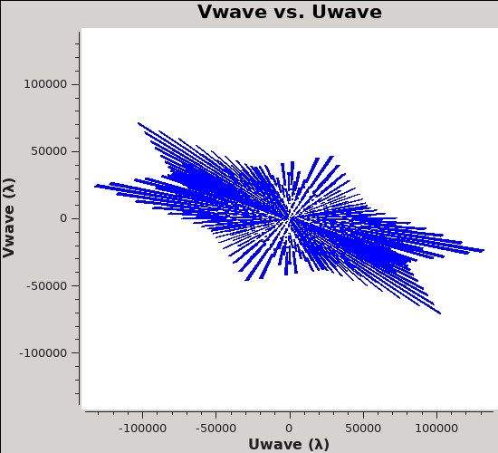
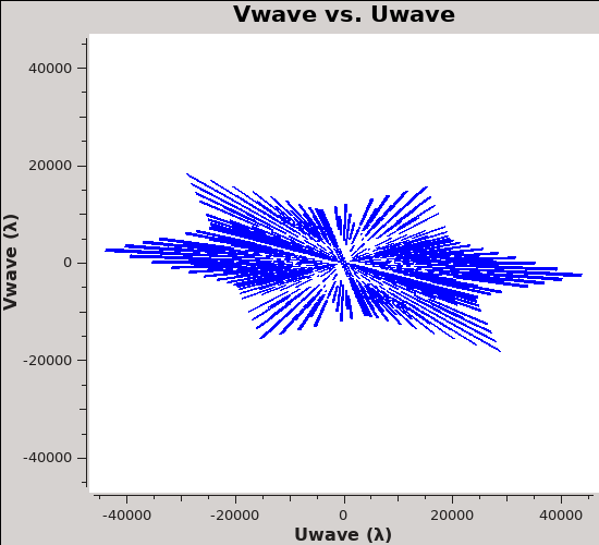
To better understand the data, let's check the uv-coverage of each of the three datasets:
# In CASA
# A-config:
plotms(vis='VLA-SgrA-Sband-Aconfig.ms',xaxis='Uwave',yaxis='Vwave')
# In CASA
# B-config
plotms(vis='VLA-SgrA-Sband-Bconfig.ms',xaxis='Uwave',yaxis='Vwave')
# In CASA
# C-config:
plotms(vis='VLA-SgrA-Sband-Cconfig.ms',xaxis='Uwave',yaxis='Vwave')
The uv-coverage plots are shown in Figures 1a-c. The u:v aspect ratio of each uv-coverage is high since Sgr A* is a very southern source. We also see that the longest baseline in each array differs by about a factor of 3, as expected, between the VLA A, B, and C configurations.
 UV-coverage of the A-configuration data. |
 UV-coverage of the B-configuration data. |
 UV-coverage of the C-configuration data. |
The next step is to create images we will then model and subtract the point source from.
We will use common cell sizes of 0.1 arcsec, which samples the A-configuration beam well and oversamples the more compact configurations. We create images of 1280 pixels on each side, and we will tclean 1000 iterations (see the VLA CASA imaging guide for more sophisticated imaging parameter choices).
# In CASA
# A-config:
tclean(vis='VLA-SgrA-Sband-Aconfig.ms', imagename='SgrA-Aonly',field='J1745-2900',
      specmode='mfs',cell='0.1arcsec',imsize=[1280,1280],niter=1000,weighting='briggs',robust=0)
# In CASA
# B-config
tclean(vis='VLA-SgrA-Sband-Bconfig.ms', imagename='SgrA-Bonly',field='J1745-2900',
      specmode='mfs',cell='0.1arcsec',imsize=[1280,1280],niter=1000,weighting='briggs',robust=0)
# In CASA
# C-config:
tclean(vis='VLA-SgrA-Sband-Cconfig.ms', imagename='SgrA-Conly',field='J1745-2900',
      specmode='mfs',cell='0.1arcsec',imsize=[1280,1280],niter=1000,weighting='briggs',robust=0)
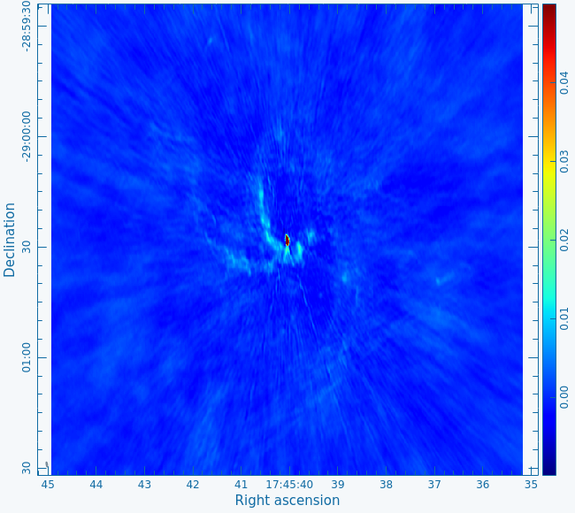
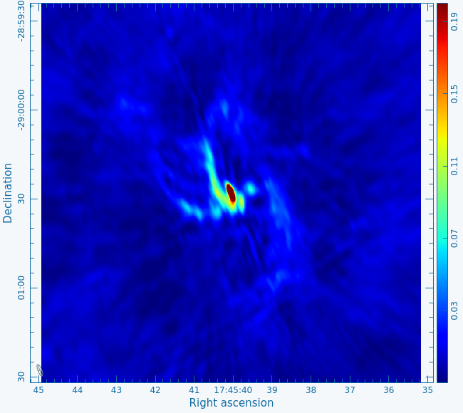
The clean images, shown in Figures 2a-c, give a first impression of the data. You can see the images using Carta in a terminal outside CASA:
# In Terminal
carta SgrA-Aonly.image
You will need to paste the path into an internet browser. Once you have opened the first image, you can use Carta menu: file -> open archive to load the others.
The basic parameters of the individual images can be checked through imhead for the spatial resolution and determining the rms when checking the statistics of empty areas within the viewer.
# In CASA
imhead('SgrA-Aonly.image')
imhead('SgrA-Bonly.image')
imhead('SgrA-Conly.image')
INFO imhead	##### Begin Task: imhead             #####
INFO imhead	imhead( imagename='SgrA-Aonly.image', mode='summary', hdkey='', hdvalue='', verbose=False )
INFO ImageMetaData
INFO ImageMetaData	Image name       : SgrA-Aonly.image
INFO ImageMetaData	Object name      : J1745-2900
INFO ImageMetaData	Image type       : PagedImage
INFO ImageMetaData	Image quantity   : Intensity
INFO ImageMetaData	Pixel mask(s)    : mask0
INFO ImageMetaData	Region(s)        : None
INFO ImageMetaData	Image units      : Jy/beam
INFO ImageMetaData	Restoring Beam   : 1.40376 arcsec, 0.400036 arcsec, 8.32141 deg
INFO ImageMetaData
INFO ImageMetaData	Direction reference : J2000
INFO ImageMetaData	Spectral  reference : LSRK
INFO ImageMetaData	Velocity  type      : RADIO
INFO ImageMetaData	Rest frequency      : 2.99881e+09 Hz
INFO ImageMetaData	Pointing center     :  17:45:40.038300  -29.00.28.068994
INFO ImageMetaData	Telescope           : EVLA
INFO ImageMetaData	Observer            : lorant sjouwerman
INFO ImageMetaData	Date observation    : 2014/05/31/09:07:58.500000
INFO ImageMetaData	Telescope position: [-1.60116e+06m, -5.04199e+06m, 3.55488e+06m] (ITRF)
INFO ImageMetaData
INFO ImageMetaData	Axis Coord Type      Name             Proj Shape Tile   Coord value at pixel         Coord incr Units
INFO ImageMetaData	-----------------------------------------------------------------------------------------------------
INFO ImageMetaData	0    0     Direction Right Ascension   SIN  1280  160  17:45:40.038   640.00      -1.000000e-01 arcsec
INFO ImageMetaData	1    0     Direction Declination       SIN  1280  160 -29.00.28.069   640.00       1.000000e-01 arcsec
INFO ImageMetaData	2    1     Stokes    Stokes                    1    1             I
INFO ImageMetaData	3    2     Spectral  Frequency                 1    1 2998809251.46     0.00 2.023871358925e+09 Hz
INFO ImageMetaData	                     Velocity                                     0     0.00      -2.023274e+05 km/s
INFO imhead	Task imhead complete. Start time: 2023-01-19 17:52:14.304617 End time: 2023-01-19 17:52:14.307656
INFO imhead	##### End Task: imhead               #####
INFO imhead	##########################################
INFO imhead	##########################################
INFO imhead	##### Begin Task: imhead             #####
INFO imhead	imhead( imagename='SgrA-Bonly.image', mode='summary', hdkey='', hdvalue='', verbose=False )
INFO ImageMetaData
INFO ImageMetaData	Image name       : SgrA-Bonly.image
INFO ImageMetaData	Object name      : J1745-2900
INFO ImageMetaData	Image type       : PagedImage
INFO ImageMetaData	Image quantity   : Intensity
INFO ImageMetaData	Pixel mask(s)    : mask0
INFO ImageMetaData	Region(s)        : None
INFO ImageMetaData	Image units      : Jy/beam
INFO ImageMetaData	Restoring Beam   : 4.12117 arcsec, 1.30587 arcsec, 20.9395 deg
INFO ImageMetaData
INFO ImageMetaData	Direction reference : J2000
INFO ImageMetaData	Spectral  reference : LSRK
INFO ImageMetaData	Velocity  type      : RADIO
INFO ImageMetaData	Rest frequency      : 2.99914e+09 Hz
INFO ImageMetaData	Pointing center     :  17:45:40.038300  -29.00.28.068994
INFO ImageMetaData	Telescope           : EVLA
INFO ImageMetaData	Observer            : lorant sjouwerman
INFO ImageMetaData	Date observation    : 2013/10/27/00:11:04.500000
INFO ImageMetaData	Telescope position: [-1.60116e+06m, -5.04199e+06m, 3.55488e+06m] (ITRF)
INFO ImageMetaData
INFO ImageMetaData	Axis Coord Type      Name             Proj Shape Tile   Coord value at pixel         Coord incr Units
INFO ImageMetaData	-----------------------------------------------------------------------------------------------------
INFO ImageMetaData	0    0     Direction Right Ascension   SIN  1280  160  17:45:40.038   640.00      -1.000000e-01 arcsec
INFO ImageMetaData	1    0     Direction Declination       SIN  1280  160 -29.00.28.069   640.00       1.000000e-01 arcsec
INFO ImageMetaData	2    1     Stokes    Stokes                    1    1             I
INFO ImageMetaData	3    2     Spectral  Frequency                 1    1 2999135410.54     0.00 2.024091446898e+09 Hz
INFO ImageMetaData	                     Velocity                                     0     0.00      -2.023274e+05 km/s
INFO imhead	Task imhead complete. Start time: 2023-01-19 17:55:34.641808 End time: 2023-01-19 17:55:34.644805
INFO imhead	##### End Task: imhead               #####
INFO imhead	##########################################
INFO imhead	##########################################
INFO imhead	##### Begin Task: imhead             #####
INFO imhead	imhead( imagename='SgrA-Conly.image', mode='summary', hdkey='', hdvalue='', verbose=False )
INFO ImageMetaData
INFO ImageMetaData	Image name       : SgrA-Conly.image
INFO ImageMetaData	Object name      : J1745-2900
INFO ImageMetaData	Image type       : PagedImage
INFO ImageMetaData	Image quantity   : Intensity
INFO ImageMetaData	Pixel mask(s)    : mask0
INFO ImageMetaData	Region(s)        : None
INFO ImageMetaData	Image units      : Jy/beam
INFO ImageMetaData	Restoring Beam   : 11.1818 arcsec, 3.98467 arcsec, 9.05307 deg
INFO ImageMetaData
INFO ImageMetaData	Direction reference : J2000
INFO ImageMetaData	Spectral  reference : LSRK
INFO ImageMetaData	Velocity  type      : RADIO
INFO ImageMetaData	Rest frequency      : 2.99912e+09 Hz
INFO ImageMetaData	Pointing center     :  17:45:40.038300  -29.00.28.068994
INFO ImageMetaData	Telescope           : EVLA
INFO ImageMetaData	Observer            : lorant sjouwerman
INFO ImageMetaData	Date observation    : 2013/08/09/04:26:49.500000
INFO ImageMetaData	Telescope position: [-1.60116e+06m, -5.04199e+06m, 3.55488e+06m] (ITRF)
INFO ImageMetaData
INFO ImageMetaData	Axis Coord Type      Name             Proj Shape Tile   Coord value at pixel         Coord incr Units
INFO ImageMetaData	-----------------------------------------------------------------------------------------------------
INFO ImageMetaData	0    0     Direction Right Ascension   SIN  1280  160  17:45:40.038   640.00      -1.000000e-01 arcsec
INFO ImageMetaData	1    0     Direction Declination       SIN  1280  160 -29.00.28.069   640.00       1.000000e-01 arcsec
INFO ImageMetaData	2    1     Stokes    Stokes                    1    1             I
INFO ImageMetaData	3    2     Spectral  Frequency                 1    1 2999123164.42     0.00 2.024083211560e+09 Hz
INFO ImageMetaData	                     Velocity                                     0     0.00      -2.023274e+05 km/s
INFO imhead	Task imhead complete. Start time: 2023-01-19 17:55:39.040544 End time: 2023-01-19 17:55:39.043544
INFO imhead	##### End Task: imhead               #####
INFO imhead	##########################################
The central point source, Sgr A*, is variable and we see this reflected in the flux density values from the images taken in the three different configurations, which were separated in observing time by several months. We can get the peak flux values from within the viewer or use the imstat task:
A-configuration: synthesized beam  1.40" x 0.40"; rms ~0.8mJy; peak flux density of Sgr A* 0.713 Jy/beam
B-configuration: synthesized beam  4.12" x 1.31"; rms ~0.7mJy; peak flux density of Sgr A* 0.691 Jy/beam
C-configuration: synthesized beam 11.18" x 3.98"; rms ~0.6mJy; peak flux density of Sgr A* 1.314 Jy/beam
Removal of the variable Sgr A* point source
We have seen in the initial images that Sgr A* is a variable source. The variability would introduce problems if a user wished to combine the datasets because the visibilities of the different sessions will reflect those variations. Cleaning would be difficult in such a situation as flux levels at different uv points (times and baselines) would not be consistent in their portion for the central point source. Therefore, we will remove the unresolved Sgr A* in each dataset. For those who are interested in having Sgr A* back in the image, we will later show how to re-introduce a nominal point source with a flux of 1Jy. It is perfectly fine, however, to image without the artificial source.
To start, we create a component list for each dataset that includes only a point source at the position of Sgr A*. To do so, we first need to find out the position of the central point source. This is performed by fitting a point source (2d-Gaussian function) to the A-configuration data, which has the largest angular resolution. We use imfit:
# In CASA
imfit(imagename='SgrA-Aonly.image',box='630,620,650,660')
The output of imfit into the logger is as follows:
Fit on SgrA-Aonly.image component 0
Position ---
       --- ra:    17:45:40.038545 +/- 0.000057 s (0.000748 arcsec along great circle)
       --- dec: -029.00.28.051094 +/- 0.004412 arcsec
       --- ra:  639.9679 +/- 0.0075 pixels
       --- dec: 640.1790 +/- 0.0441 pixels
We will use RA (J2000) =17h45m40.039s and DEC (J2000) = -29d00'28.05" as the central position of Sgr A* for all three configurations; it might be advisable to fit each dataset separately in case the peak may slightly shift. In this case, a single position works for all of our three data sets.
The component list will be inserted as a MODEL column into the respective MS via ft. Task uvsub will then be used to subtract the point source model from the CORRECTED data column. Since there's no CORRECTED column to start with, uvsub will initially copy the DATA column to the CORRECTED column, then subtract. Note that running uvsub twice will oversubtract; we recommend to create backup copies of the previous datasets before subtracting Sgr A*:
# In a Terminal
cp -r VLA-SgrA-Sband-Aconfig.ms VLA-SgrA-Sband-Aconfig-sub.ms
cp -r VLA-SgrA-Sband-Bconfig.ms VLA-SgrA-Sband-Bconfig-sub.ms
cp -r VLA-SgrA-Sband-Cconfig.ms VLA-SgrA-Sband-Cconfig-sub.ms
Let's start with the A-configuration data and create a component list of a point source with a flux of 0.712 Jy at a position of RA (J2000) =17h45m40.038547s and DEC (J2000) = -29d00'28.051226" (more examples of component lists are provided in the CASA guide Create a Component List for Selfcal):
# In CASA
cl.addcomponent(flux=0.713, fluxunit='Jy',shape='point', dir='J2000 17:45:40.039 -29.00.28.05')
cl.rename('component-SgrA-A.cl')
cl.close()
(We have used the CASA coordinate convention with colons for h:m:s and dots for d.m.s.)
The component list is now stored in the file 'component-SgrA-A.cl' and we will use it to populate the MODEL column via ft:
# In CASA
ft(vis='VLA-SgrA-Sband-Aconfig-sub.ms', complist='component-SgrA-A.cl', usescratch=True)
At this step the MODEL column is created.
Finally, we subtract the MODEL from the DATA/CORRECTED_DATA with uvsub. This task will also create CORRECTED as it does not exist yet:
# In CASA
uvsub(vis='VLA-SgrA-Sband-Aconfig-sub.ms')
Note that to revert back to the original state you can use task clearcal to reset the MODEL column and to set CORRECTED to be identical with DATA (thus undoing the source subtraction).
uvsub in CASA 6.4.1 has a bug and will show an error message like 'name 'vis' is not defined'. The task still appears to work correctly though, just the history entry seems to be compromised.
Let's repeat the steps for B-configuration, now using a flux of 0.691 Jy. Although a separate fit would be even better, the subtraction also works well when using the A-configuration position:
# In CASA
cl.addcomponent(flux=0.691, fluxunit='Jy',shape='point', dir='J2000 17:45:40.039 -29.00.28.05')
cl.rename('component-SgrA-B.cl')
cl.close()
#
ft(vis='VLA-SgrA-Sband-Bconfig-sub.ms', complist='component-SgrA-B.cl', usescratch=True)
#
uvsub(vis='VLA-SgrA-Sband-Bconfig-sub.ms')
And for C-configuration we subtract a point source of 1.314 Jy (note that the central flux includes some extended emission, but is still dominated by Sgr A*):
# In CASA
cl.addcomponent(flux=1.314, fluxunit='Jy',shape='point', dir='J2000 17:45:40.039 -29.00.28.05')
cl.rename('component-SgrA-C.cl')
cl.close()
#
ft(vis='VLA-SgrA-Sband-Cconfig-sub.ms', complist='component-SgrA-C.cl', usescratch=True)
#
uvsub(vis='VLA-SgrA-Sband-Cconfig-sub.ms')
Image the three data sets with Sgr A* removed. We run tclean, but since the point source is removed, we only do 500 iterations for A and B configurations, and 200 iterations for the C configuration data to avoid cleaning into the noise:
# In CASA
# A-config:
tclean(vis='VLA-SgrA-Sband-Aconfig-sub.ms', imagename='SgrA-Aonly-noPNT',field='J1745-2900',
      specmode='mfs',cell='0.1arcsec',imsize=[1280,1280],niter=500,weighting='briggs',robust=0)
# In CASA
# B-config:
tclean(vis='VLA-SgrA-Sband-Bconfig-sub.ms', imagename='SgrA-Bonly-noPNT',field='J1745-2900',
      specmode='mfs',cell='0.1arcsec',imsize=[1280,1280],niter=500,weighting='briggs',robust=0)
# In CASA
# C-config:
tclean(vis='VLA-SgrA-Sband-Cconfig-sub.ms', imagename='SgrA-Conly-noPNT',field='J1745-2900',
      specmode='mfs',cell='0.1arcsec',imsize=[1280,1280],niter=200,weighting='briggs',robust=0)
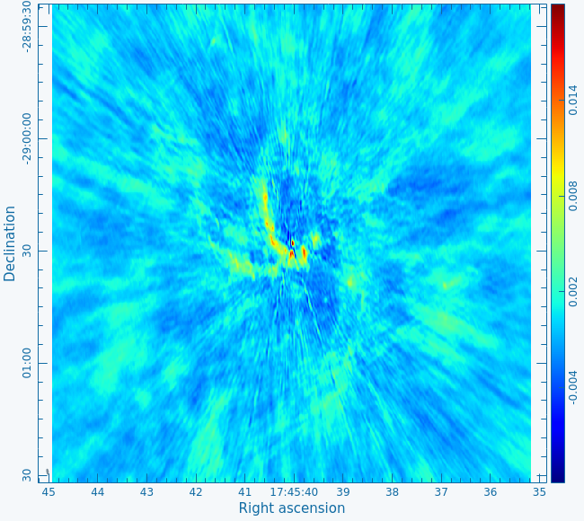
As expected, the images without the point sources as shown in Figures 3a-c look similar to those in Figures 2a-c. but with the central point source removed. Since we cleaned a given number of iterations, some differences are visible, particularly for C-configuration. This is expected.
Inserting an artificial Point Source for Sgr A*
We can add a point source with a canonical flux density of 1 Jy to bring back Sgr A*. Again create a component list and use ft to attach the source model. Using uvsub with reverse=True will add instead of subtract the MODEL to DATA/CORRECTED. This step can be skipped when Sgr A* is not required. When the data are going to be self-calibrated, we recommend to not introduce an artificial source during the calibration steps as it has no phase errors imprinted. For this example, we re-introduce Sgr A* to the A-configuration dataset. First copy the dataset to the dataset the point source will be added to.
# In a Terminal
cp -r VLA-SgrA-Sband-Aconfig-sub.ms VLA-SgrA-Sband-Aconfig-addPNT.ms
Create a component list with a 1 Jy point source at the previously derived position of Sgr A*.
# In CASA
cl.addcomponent(flux=1, fluxunit='Jy',shape='point', dir='J2000 17:45:40.039 -29.00.28.05')
cl.rename('component-SgrA.cl')
cl.close()
Insert the point source component into the model column with ft and add it to the data with uvsub to the MS:
# In CASA
ft(vis='VLA-SgrA-Sband-Aconfig-addPNT.ms', complist='component-SgrA.cl', usescratch=True)
#
uvsub(vis='VLA-SgrA-Sband-Aconfig-addPNT.ms',reverse=True)
After inserting Sgr A* back into the dataset we image the measurement set once again.
# In CASA
tclean(vis=['VLA-SgrA-Sband-Aconfig-addPNT.ms'],
      imagename='GC-addPNT',field='J1745-2900',specmode='mfs',cell='0.1arcsec',imsize=[1280,1280],niter=5000,
      threshold='5mJy',weighting='briggs',robust=0)
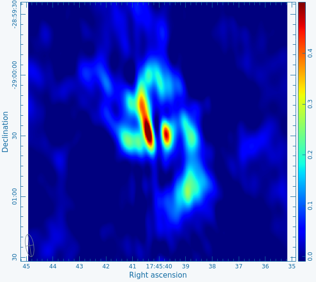
In Figure 4 we show the resulting image on the same scales as in Figure 2a. As expected the main difference is the added point source but some differences due to the tclean algorithm are also visible. Again, one can improve the images as described above.
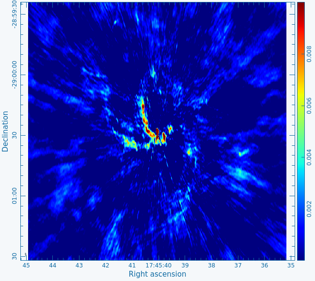 Combined image with a steady point source re-added. To get a similar image, in the Viewer task, click on the Wrench icon and in the Basic setting change the data range to [0, 0.1] |
Last checked on CASA Version 6.4.1
