IRAS16293 Band9 - Imaging for CASA 5.1: Difference between revisions
| Line 103: | Line 103: | ||
field='',xaxis='uvdist', yaxis='amp', | field='',xaxis='uvdist', yaxis='amp', | ||
spw='1', avgchannel='3840',coloraxis='field', | spw='1', avgchannel='3840',coloraxis='field', | ||
iteraxis='field',yselfscale=True) | iteraxis='field',yselfscale=True,showgui=True) | ||
</source> | </source> | ||
| Line 115: | Line 115: | ||
field='',xaxis='uvdist', yaxis='amp', | field='',xaxis='uvdist', yaxis='amp', | ||
spw='', avgchannel='3840',coloraxis='field', | spw='', avgchannel='3840',coloraxis='field', | ||
iteraxis='spw') | iteraxis='spw',showgui=True) | ||
</source> | </source> | ||
| Line 133: | Line 133: | ||
spw='', avgtime='1e8',avgscan=True,coloraxis='corr', | spw='', avgtime='1e8',avgscan=True,coloraxis='corr', | ||
avgchannel='',iteraxis='spw',ydatacolumn='data', | avgchannel='',iteraxis='spw',ydatacolumn='data', | ||
xselfscale=True,yselfscale=True) | xselfscale=True,yselfscale=True,showgui=True) | ||
</source> | </source> | ||
| Line 200: | Line 200: | ||
plotms(vis='IRAS16293_Band9.fixed.CONT.msAVG', | plotms(vis='IRAS16293_Band9.fixed.CONT.msAVG', | ||
xaxis='time', yaxis='amp',field='',iteraxis='field', | xaxis='time', yaxis='amp',field='',iteraxis='field', | ||
spw='', avgchannel='4000',coloraxis='field', | spw='', avgchannel='4000',coloraxis='field',showgui=True, | ||
ydatacolumn='model',xselfscale=True,yselfscale=True) | ydatacolumn='model',xselfscale=True,yselfscale=True) | ||
</source> | </source> | ||
| Line 221: | Line 221: | ||
plotcal(caltable='cont_pcal1',xaxis='time',yaxis='phase', | plotcal(caltable='cont_pcal1',xaxis='time',yaxis='phase', | ||
spw='',iteration='antenna',subplot=511,plotrange=[0,0,-80,80], | spw='',iteration='antenna',subplot=511,plotrange=[0,0,-80,80], | ||
antenna='',timerange='') | antenna='',timerange='',showgui=True) | ||
# The phases are remarkably stable for Band 9! | # The phases are remarkably stable for Band 9! | ||
| Line 290: | Line 290: | ||
plotcal(caltable='cont_pcal2',xaxis='time',yaxis='phase', | plotcal(caltable='cont_pcal2',xaxis='time',yaxis='phase', | ||
spw='',iteration='antenna',subplot=511,plotrange=[0,0,-80,80], | spw='',iteration='antenna',subplot=511,plotrange=[0,0,-80,80], | ||
antenna='',timerange='') | antenna='',timerange='',showgui=True) | ||
# Applying results to the data | # Applying results to the data | ||
| Line 345: | Line 345: | ||
plotcal(caltable='cont_apcal',xaxis='time',yaxis='amp', | plotcal(caltable='cont_apcal',xaxis='time',yaxis='amp', | ||
spw='',iteration='antenna',subplot=511,plotrange=[0,0,0.5,2], | spw='',iteration='antenna',subplot=511,plotrange=[0,0,0.5,2], | ||
antenna='',timerange='') | antenna='',timerange='',showgui=True) | ||
# and applying to the data | # and applying to the data | ||
Revision as of 13:27, 28 September 2018
WARNING: On June 15, 2012 the calibration guide and the final data products (calibrated science
data: IRAS16293_Band9_CalibratedMS_FIXED.tgz and reference images: IRAS16293_Band9_ReferenceImages_FIXED.tgz))
were changed to correct for a 1.2" position error in the phase calibrator (1625-254). Without
correction, the science images will suffer from a similar offset.
Overview
This section of the casa guide continues from IRAS16293_Band9_-_Calibration_for_CASA_5.1 . If you completed the calibration section, then you already have the final calibrated dataset. If you just started to work on this IRAS16293 B9 data, you can download the fully calibrated dataset IRAS16293_Band9_CalibratedMS from
This casa guide covers imaging of both continuum and spectral lines of IRAS16293 Band 9. This guide requires CASA 5.1.1. In this casa guide you will also need the Analysis Utils package, so make sure you have it imported into CASA.
Confirm your version of CASA
This guide has been written for CASA release 5.1.1. Please confirm your version before proceeding.
# In CASA
import casadef
version = casadef.casa_version
print "You are using " + version
if (version < '5.1.1'):
    print "YOUR VERSION OF CASA IS TOO OLD FOR THIS GUIDE."
    print "PLEASE UPDATE IT BEFORE PROCEEDING."
else:
    print "Your version of CASA is appropriate for this guide."
Install Analysis Utilities
Analysis Utilities (or analysisUtils for short) is a small set of Python scripts that provide a number of analysis and plotting utilities for ALMA data reduction. This guide uses a few of these utilities. They are very easy to install (just download and untar). See
http://casaguides.nrao.edu/index.php?title=Analysis_Utilities
for a full description and download instructions. If you do not wish to do this, see the CASA 3.3 version of the guide linked at the top of this page for alternative (but slow) plotting options. Analysis Utilities are updated frequently so if its been a while since you installed it, its probably worth doing it again. If you are at an ALMA site or ARC, the analysis utilities are probably already installed and up to date.
List the contents of the Data
Before we start with the imaging itself, do a listobs to the calibrated dataset, so you can check that everything is ok. Make sure there are 4 observations, 7 fields, and 4 spectral windows (spws).
# listobs to check data
listobs(vis='IRAS16293_Band9.fixed.rebin.ms',
        listfile='IRAS16293_Band9.fixed.rebin.ms.listobs',verbose=False)
You should see the next information in the .listobs file.
  Telescope Observation Date    Observer       Project
  ALMA      [                   4.84128e+09, 4.84129e+09]dgarcia        uid://A002/X3cd6b2/X53
  ALMA      [                   4.84135e+09, 4.84136e+09]dgarcia        uid://A002/X3cd6b2/X53
  ALMA      [                   4.84137e+09, 4.84137e+09]dgarcia        uid://A002/X3cd6b2/X53
  ALMA      [                   4.84137e+09, 4.84138e+09]dgarcia        uid://A002/X3cd6b2/X53
Data records: 52996       Total elapsed time = 98524.9 seconds
   Observed from   16-Apr-2012/08:27:40.4   to   17-Apr-2012/11:49:45.3 (UTC)

Fields: 7
  ID   Code Name                RA               Decl           Epoch   SrcId      nRows
  0    none IRAS16293-2422-a    16:32:22.992000 -24.28.36.00000 J2000   0           7812
  1    none IRAS16293-2422-a    16:32:22.479253 -24.28.36.00000 J2000   0           7821
  2    none IRAS16293-2422-a    16:32:22.735626 -24.28.36.00000 J2000   0           7821
  3    none IRAS16293-2422-a    16:32:22.735626 -24.28.32.50000 J2000   0           7821
  4    none IRAS16293-2422-a    16:32:22.479253 -24.28.29.00000 J2000   0           7439
  5    none IRAS16293-2422-a    16:32:22.735626 -24.28.29.00000 J2000   0           7141
  6    none IRAS16293-2422-a    16:32:22.992000 -24.28.29.00000 J2000   0           7141
Spectral Windows:  (4 unique spectral windows and 1 unique polarization setups)
  SpwID  Name                           #Chans   Frame   Ch0(MHz)  ChanWid(kHz)  TotBW(kHz) CtrFreq(MHz) BBC Num  Corrs
  0      ALMA_RB_09#BB_1#SW-01#FULL_RES   3840   TOPO  703312.744       488.281   1875000.0 704250.0000        1  XX  YY
  1      ALMA_RB_09#BB_2#SW-01#FULL_RES   3840   TOPO  692237.256      -488.281   1875000.0 691300.0000        2  XX  YY
  2      ALMA_RB_09#BB_3#SW-01#FULL_RES   3840   TOPO  690437.256      -488.281   1875000.0 689500.0000        3  XX  YY
  3      ALMA_RB_09#BB_4#SW-01#FULL_RES   3840   TOPO  688437.256      -488.281   1875000.0 687500.0000        4  XX  YY
Antennas: 13 'name'='station'
   ID=   0-3: 'DA41'='A003', 'DA43'='A075', 'DA47'='A026', 'DV02'='A077',
   ID=   4-8: 'DV03'='A137', 'DV07'='A076', 'DV09'='A046', 'DV10'='A071',
   ID=  9-13: 'DV12'='A011', 'DV13'='A072', 'DV14'='A025', 'DV17'='A138',
   ID= 14-14: 'DV18'='A053'
Continuum Emission Imaging
As shown in Figure 2 of IRAS16293Band9, these observations have a 7 pointing mosaic, which you can visualize with the next command (see also Figure 1).
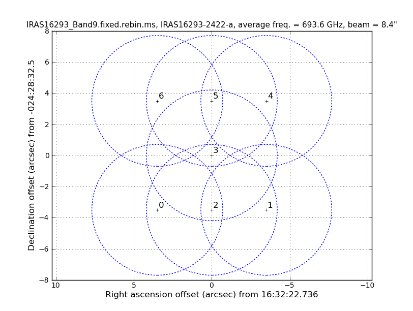
# Make a plot of the mosaic pattern with field ids identified
au.plotmosaic(vis='IRAS16293_Band9.fixed.rebin.ms',sourceid='0',
              doplot=True,figfile='mosaic_pattern.png')
You might wonder which of these pointings or fields have stronger line emission. You can determine this by running the next command. We set spw='1' which contains CO (6-5), and you can check all the plots for all the fields by just hitting the arrow for "next". Also see Figure 2 for an example of the output.
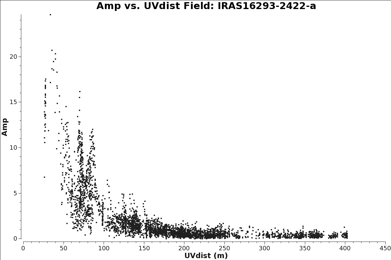
# See which mosaic fields have the brightest line emission
plotms(vis='IRAS16293_Band9.fixed.rebin.ms',
       field='',xaxis='uvdist', yaxis='amp',
       spw='1', avgchannel='3840',coloraxis='field',
       iteraxis='field',yselfscale=True,showgui=True)
Another way to visualize the uv-amp distribution is with the next plotms. This will load all the fields for pointing into the plot, and you can change interactively between the spws using the appropriate button in plotms. See Figure 3 for a plot of spw 0. Remember you can use the locate and zoom features to find more information about each plotted point.
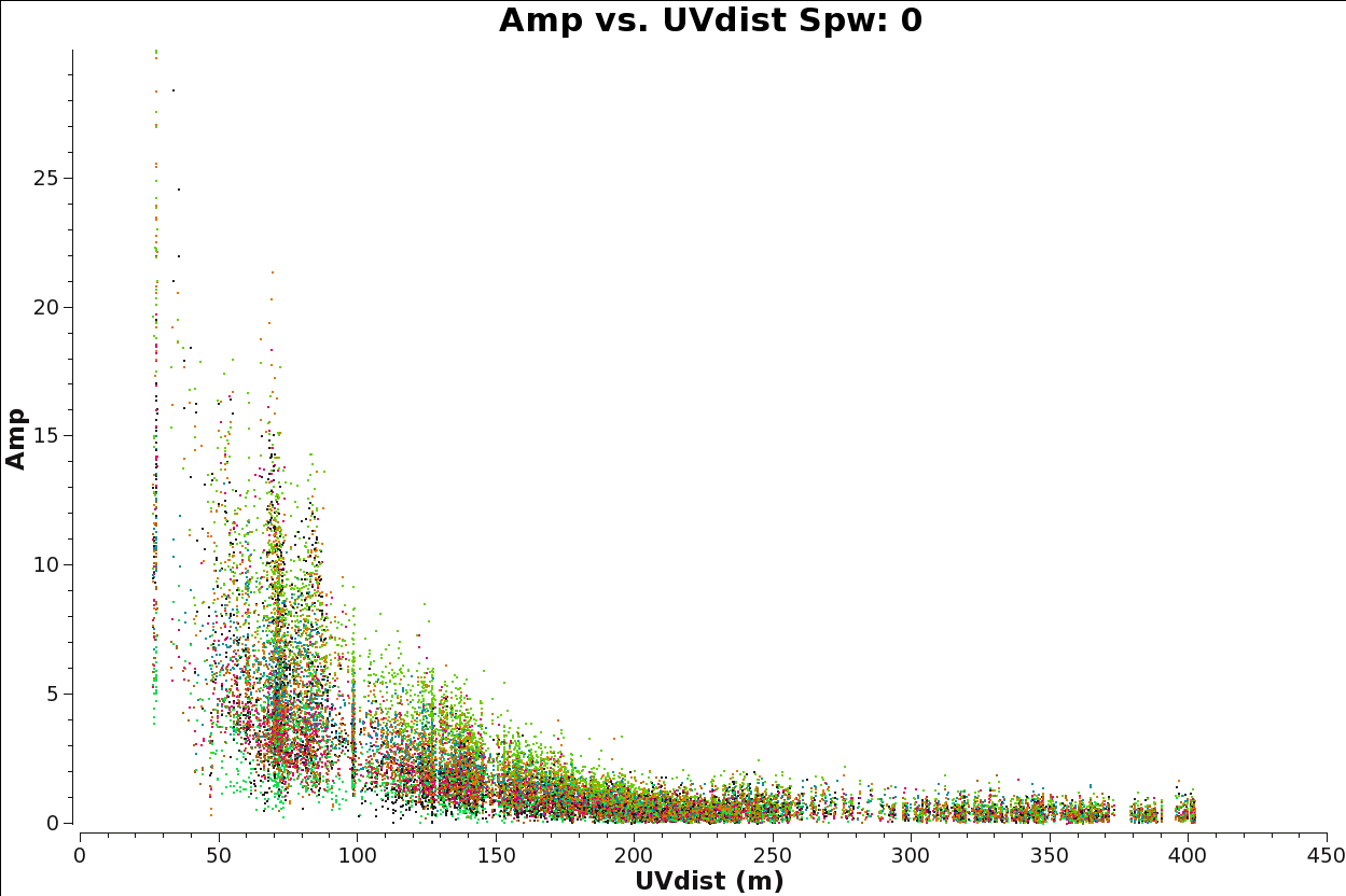
# Iterate over spws all fields
plotms(vis='IRAS16293_Band9.fixed.rebin.ms',
       field='',xaxis='uvdist', yaxis='amp',
       spw='', avgchannel='3840',coloraxis='field',
       iteraxis='spw',showgui=True)
In order to properly measure the amount of CO(6-5) emission, we need to note the channels that do not present line emission. We will use these channels to image the continuum and subtract the continuum prior to line imaging. To identify them we can plot the amplitude vs frequency for all the spectral windows.
Figure 4 shows the output from the next command for spw 0 (field 3). Note: If you are using the calibrated data from the science portal, or if you calibrated the raw data yourself following the steps in the IRAS16293_Band9_-_Calibration_for_CASA_5.1 CASA Guide, you now have a set of data which were split so the calibrated data now reside in the "data" column of the new measurement set. Therefore the following call to plotms must specify ydatacolumn = "data". If you never performed the split, the calibrated data would have been accessed from the "corrected" column of the old, unsplit, measurement set. Those who have used previous versions of CASA should note that in those older versions, plotms would default to using the "data" column if there were no data in the "corrected" column and one specified ydatacolumn="corrected".
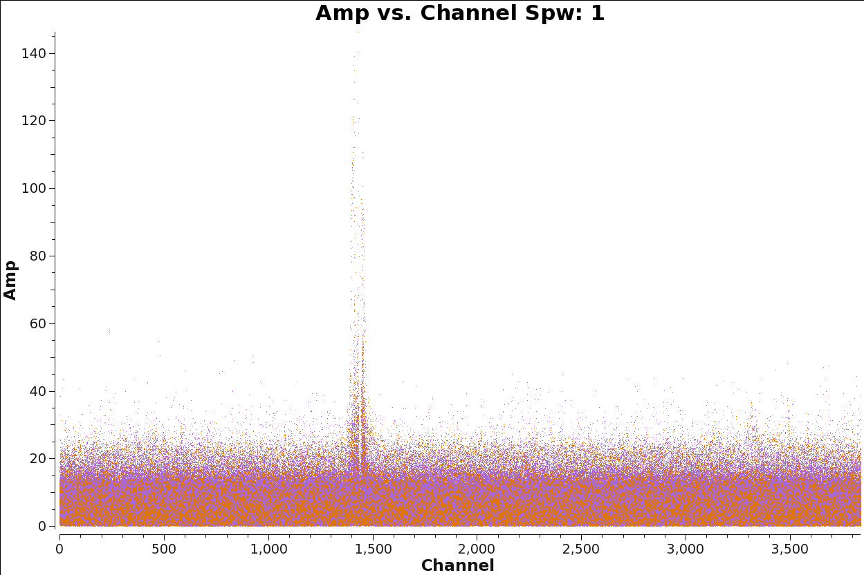
# Select Channels for uvcontsub. Average every 8 channels for
# increased S/N.

plotms(vis='IRAS16293_Band9.fixed.rebin.ms',
       xaxis='channel', yaxis='amp',field='3',
       spw='', avgtime='1e8',avgscan=True,coloraxis='corr',
       avgchannel='',iteraxis='spw',ydatacolumn='data',
       xselfscale=True,yselfscale=True,showgui=True)
Using the plots from the previous command you can select a block of channels that are free of strong line emission. To do this in the most rigorous way, you would first need to make dirty image cubes and then examine the spectra on and near the continuum sources, because many more weaker lines will become apparent in the cubes. See Image_Continuum#Create_an_Averaged_Continuum_MS for more detailed instructions and commands to do this. Here we provide you with the channel selection we used for continuum emission.
The next flagmanager command will save the flags state in case you might need to re-do the steps from this point.
flagmanager(vis='IRAS16293_Band9.fixed.rebin.ms',mode='save',versionname='Original')
Now we will flag the channels identified to have line emission, so we will be ready to proceed with the continuum imaging.
# flagging the line channels
flagdata(vis='IRAS16293_Band9.fixed.rebin.ms',
         spw='0:1700~2500,1:400~500;1100~1900;3000~3450,2:1700~2200;3100~3839,3:0~800;1600~2900;3300~3839',action='apply', flagbackup=False)
To help clean to be faster, you can average 200 channels, as you do not need to have a high spectral resolution for continuum imaging. See Image_Continuum#Create_an_Averaged_Continuum_MS for more information on choosing the ideal width to average over while avoiding bandwidth smearing.
split(vis='IRAS16293_Band9.fixed.rebin.ms',
      outputvis='IRAS16293_Band9.fixed.CONT.msAVG',field='',
      datacolumn='data',width=200,spw='0~3:20~3819')
Clean and self-calibrate the continuum
Now we proceed with the cleaning itself. For the tclean task you will need to choose the right cell size, map size, etc. Below are the parameters that were used in this casaguide. For further discussion on imaging parameters, see Image_Continuum#Image_Parameters. Note that the command will be interactive and you will have to set the cleaning boxes. For a basic guide to cleaning, see First_Look_at_Imaging.
Since we will be self-calibrating this dataset, we will be conservative in this first tclean run. Mask only the brightest emission, and only run for one or two major cycles to create a first, initial model of the source emission.
# cleaning 1
os.system('rm -rf *CONTIN*')
tclean(vis='IRAS16293_Band9.fixed.CONT.msAVG',
     imagename='IRAS16293_Band9.fixed.CONTIN',
     spw='0~3',field='',phasecenter=3,
     specmode='mfs',gridder='mosaic',
     imsize=720,cell='0.028arcsec',
     interactive=True,deconvolver='hogbom',nterms=1,
     weighting='briggs',robust=0.5,savemodel='modelcolumn',
     niter=1000, threshold='75.0mJy')
tclean only saves the model after a major cycle. This is essential to do self-calibration. tclean should warn you about this after you exit. The following command is set up to save the model column. This step will be unnecessary in CASA 5.3 and later.
# save model column
tclean(vis='IRAS16293_Band9.fixed.CONT.msAVG',
     imagename='IRAS16293_Band9.fixed.CONTIN',
     spw='0~3',field='',phasecenter=3,
     specmode='mfs',gridder='mosaic',
     imsize=720,cell='0.028arcsec',
     interactive=True,deconvolver='hogbom',nterms=1,
     weighting='briggs',robust=0.5,savemodel='modelcolumn',
     niter=0, threshold='0.3mJy',calcres=False,calcpsf=False)
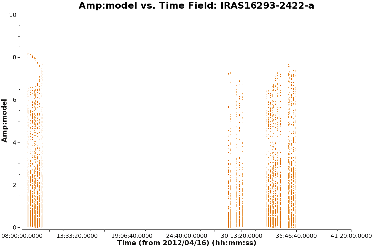
It is important to check if all fields have some emission in the model data column, if not, or if it is very weak you would want to exclude those fields from the gaincal below. Because the bright Source B is within the primary beam of all the observed fields, all fields have strong emission present in the image model. In Figure 5 you can see an example for the output from next command. If there was no signal for one of the fields, you would see values at 0 amplitude.
# checking the model data for all the fields
plotms(vis='IRAS16293_Band9.fixed.CONT.msAVG',
      xaxis='time', yaxis='amp',field='',iteraxis='field',
      spw='', avgchannel='4000',coloraxis='field',showgui=True,
      ydatacolumn='model',xselfscale=True,yselfscale=True)
Now we proceed with gaincal to perform self calibration (for phases) on the data. Even with minsnr=3.0 there will be some failed solutions. For more information on self-calibration see First_Look_at_Self_Calibration.
# get one scan per field
os.system('rm -rf cont_pcal1')
gaincal(vis='IRAS16293_Band9.fixed.CONT.msAVG',caltable='cont_pcal1',gaintype='T',
        refant='DV14',calmode='p',combine='',spw='',field='',
        solint='inf',minsnr=3.0,minblperant=4)
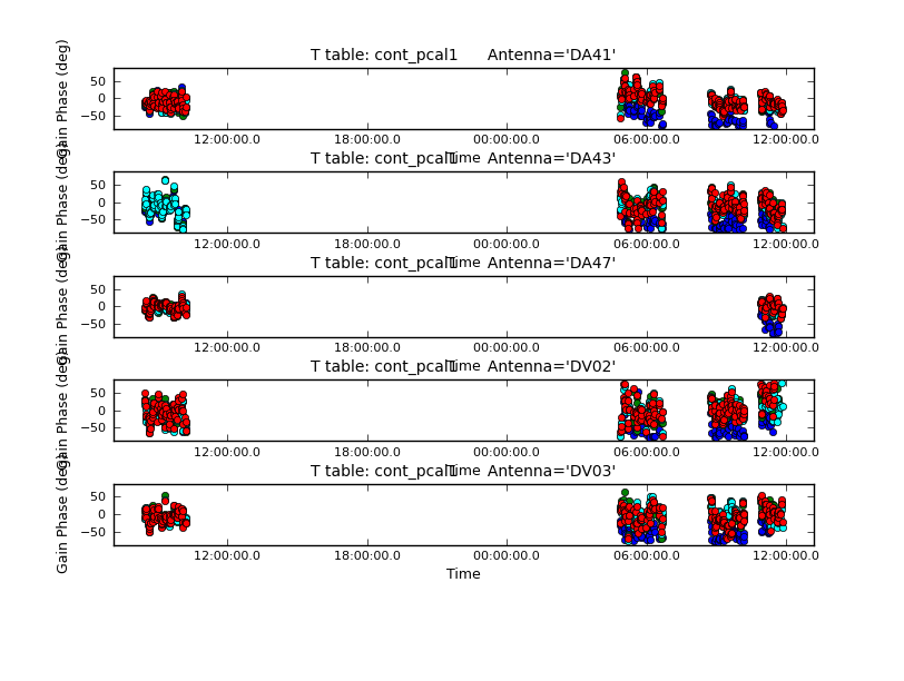
The solutions for five antennas are shown in Figure 6, and are produced with the next plotcal. Be sure to check all the antennas. Look for apparent large corrections or wrapping. Remember these are the corrections, not the data. Note any antennas that seem concerning.
plotcal(caltable='cont_pcal1',xaxis='time',yaxis='phase',
        spw='',iteration='antenna',subplot=511,plotrange=[0,0,-80,80],
        antenna='',timerange='',showgui=True)

# The phases are remarkably stable for Band 9!
Before applying the calibrations to the data, we will again save the flags state in case we want to re-do the steps from this point. To restore the flags, set 'mode='restore'.
flagmanager(vis='IRAS16293_Band9.fixed.rebin.CONT.msAVG',mode='save',versionname='Original')
We then apply the table to the data. We will check the solutions by cleaning the data again and comparing the self-calibrated and non-self-calibrated data.
# application of the table
applycal(vis='IRAS16293_Band9.fixed.CONT.msAVG',spwmap=[],spw='',
       gaintable=['cont_pcal1'],calwt=False,flagbackup=False)
Now you are ready for the second cleaning. For this one we are using the mask resulting from the previous cleaning. In the next blocks of commands we will repeat this process (clean, viewer, gaincal, plotcal, applycal, clean, etc.) to improve the overall quality of the image. You can add to your clean mask as you go, but be careful to avoid adding sidelobe emission as real structure.
# cleaning 2
os.system('rm -rf *CONTIN_P1*')
tclean(vis='IRAS16293_Band9.fixed.CONT.msAVG',
     imagename='IRAS16293_Band9.fixed.CONTIN_P1',
     mask='IRAS16293_Band9.fixed.CONTIN.mask',
     spw='0~3',field='',phasecenter=3,
     specmode='mfs',gridder='mosaic',
     imsize=720,cell='0.028arcsec',
     interactive=True,deconvolver='hogbom',nterms=1,
     weighting='briggs',robust=0.5,savemodel='modelcolumn',
     niter=1000, threshold='50.0mJy')

# visualize the image
imview (raster=[{'file':'IRAS16293_Band9.fixed.CONTIN.image',
                 'range': [-0.01,0.5]},
                {'file': 'IRAS16293_Band9.fixed.CONTIN_P1.image',
                 'range': [-0.01,0.5]}])
Make sure the model column is saved again.
# save model column
tclean(vis='IRAS16293_Band9.fixed.CONT.msAVG',
     imagename='IRAS16293_Band9.fixed.CONTIN_P1',
     spw='0~3',field='',phasecenter=3,
     specmode='mfs',gridder='mosaic',
     imsize=720,cell='0.028arcsec',
     interactive=True,deconvolver='hogbom',nterms=1,
     weighting='briggs',robust=0.5,savemodel='modelcolumn',
     niter=0, threshold='0.3mJy',calcres=False,calcpsf=False)
The image "IRAS16293_Band9.fixed.CONTIN_P1.image" should have 2 very clearly defined regions of emission, moreso then the first clean run "IRAS16293_Band9.fixed.CONTIN.image," following self-calibration.
Second gaincal step for self calibration.
# second self-cal
os.system('rm -rf cont_pcal2')
gaincal(vis='IRAS16293_Band9.fixed.CONT.msAVG',caltable='cont_pcal2',gaintype='T',
        refant='DV14',calmode='p',combine='',spw='',field='',
        solint='inf',minsnr=3.0,minblperant=4)

#Checking the table
plotcal(caltable='cont_pcal2',xaxis='time',yaxis='phase',
        spw='',iteration='antenna',subplot=511,plotrange=[0,0,-80,80],
        antenna='',timerange='',showgui=True)

# Applying results to the data
applycal(vis='IRAS16293_Band9.fixed.CONT.msAVG',spwmap=[],spw='',
       gaintable=['cont_pcal2'],calwt=False,flagbackup=False)
We continue with the next cleaning.
# Cleaning 3
os.system('rm -rf *CONTIN_P2*')
tclean(vis='IRAS16293_Band9.fixed.CONT.msAVG',
     imagename='IRAS16293_Band9.fixed.CONTIN_P2',
     spw='0~3',field='',phasecenter=3,
     specmode='mfs',gridder='mosaic',
     imsize=720,cell='0.028arcsec',
     interactive=True,deconvolver='hogbom',nterms=1,
     weighting='briggs',robust=0.5,savemodel='modelcolumn',
     niter=1000, threshold='40.0mJy')

# Save model
tclean(vis='IRAS16293_Band9.fixed.CONT.msAVG',
     imagename='IRAS16293_Band9.fixed.CONTIN_P2',
     spw='0~3',field='',phasecenter=3,
     specmode='mfs',gridder='mosaic',
     imsize=720,cell='0.028arcsec',
     interactive=True,deconvolver='hogbom',nterms=1,
     weighting='briggs',robust=0.5,savemodel='modelcolumn',
     niter=0, threshold='0.3mJy',calcres=False,calcpsf=False)

# to view the resulting image
imview (raster=[{'file':'IRAS16293_Band9.fixed.CONTIN_P1.image',
                 'range': [-0.01,0.5]},
                {'file': 'IRAS16293_Band9.fixed.CONTIN_P2.image',
                 'range': [-0.01,0.5]}])

# There is very little change, the bold could try another iteration using a shorter
# solint phase self-cal. For now, moving on to amplitude.
Next iteration with gaincal, now using amplitude and phase for "calmode".
# For amplitude self-cal we only want to get one solution per spw, per dataset
os.system('rm -rf cont_apcal')
gaincal(vis='IRAS16293_Band9.fixed.CONT.msAVG',caltable='cont_apcal',gaintype='T',
        refant='DV14',calmode='ap',combine='scan,field',spw='',field='',
        solint='8000s',minsnr=3.0,minblperant=4,gaintable='cont_pcal2')

# ploting the table
plotcal(caltable='cont_apcal',xaxis='time',yaxis='amp',
        spw='',iteration='antenna',subplot=511,plotrange=[0,0,0.5,2],
        antenna='',timerange='',showgui=True)

# and applying to the data
applycal(vis='IRAS16293_Band9.fixed.CONT.msAVG',spwmap=[],spw='',
       gaintable=['cont_pcal2','cont_apcal'],calwt=False,flagbackup=False)

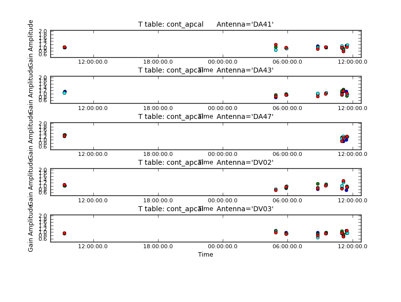
# A large correction is present for the 2nd dataset. This amplitude
# error was causing many of the artifacts noticeable in the previous
# images.
Continuing the final cleaning step. We will re-use the mask from the P2 image.
# Cleaning 4
os.system('rm -rf *CONTIN_AP*')
tclean(vis='IRAS16293_Band9.fixed.CONT.msAVG',
     imagename='IRAS16293_Band9.fixed.CONTIN_AP',
     spw='0~3',field='',phasecenter=3,
     specmode='mfs',gridder='mosaic',
     imsize=720,cell='0.028arcsec',
     interactive=True,deconvolver='hogbom',nterms=1,
     mask='IRAS16293_Band9.fixed.CONTIN_P2.mask',
     weighting='briggs',robust=0.5,savemodel='modelcolumn',
     niter=1000, threshold='40.0mJy',pbcor=True)

# Save model
tclean(vis='IRAS16293_Band9.fixed.CONT.msAVG',
     imagename='IRAS16293_Band9.fixed.CONTIN_AP',
     spw='0~3',field='',phasecenter=3,
     specmode='mfs',gridder='mosaic',
     imsize=720,cell='0.028arcsec',
     interactive=True,deconvolver='hogbom',nterms=1,
     weighting='briggs',robust=0.5,savemodel='modelcolumn',
     niter=0, threshold='0.3mJy',calcres=False,calcpsf=False)

# and to view the image
imview (raster=[{'file':'IRAS16293_Band9.fixed.CONTIN_P2.image',
                 'range': [-0.01,0.5]},
                {'file': 'IRAS16293_Band9.fixed.CONTIN_AP.image',
                 'range': [-0.01,0.5]}])
We will use immath to cut out a sub-region of the cube because the area covered is large compared to the area of interest, and we want to keep the file size of the result as small as possible.
# in CASA
immath('IRAS16293_Band9.fixed.CONTIN_AP.image.pbcor',outfile='IRAS16293_Band9.fixed.CONTIN_AP.image.subim.pbcor',
        box='221,160,493,430',expr='IM0')
Note that no GUI will appear in the next imview command because we have specified an output file.
# check the image
imview (raster=[{'file': 'IRAS16293_Band9.fixed.CONTIN_AP.image.subim.pbcor',
                 'range': [-0.01,1.5],'colorwedge':True}],
        out='IRAS16293_Band9.fixed.CONTIN_AP.image.pbcor.png')
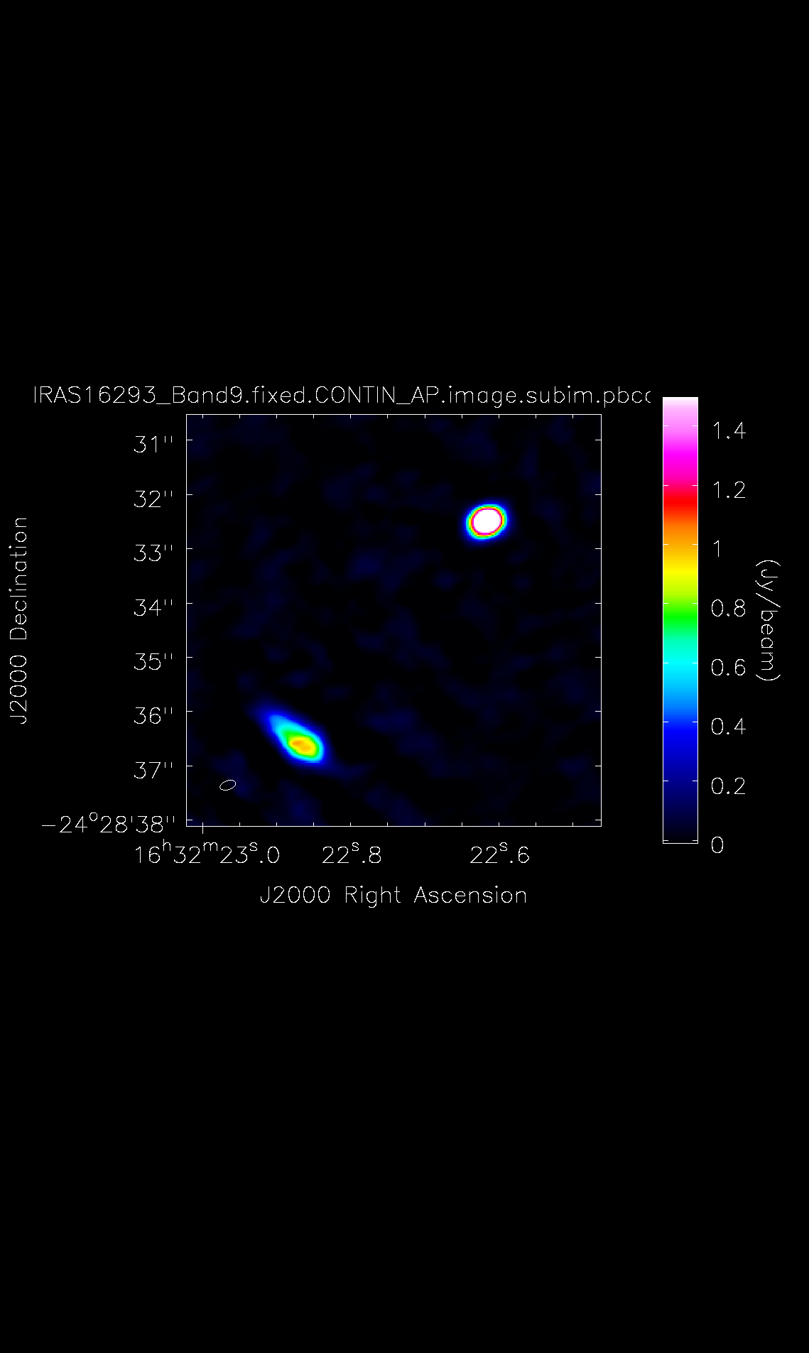
In Figure 7 we show the final image of the self-calibration process. Source A is the weaker source to the SE and Source B is the stronger source to the NW. The rms noise is about 18 mJy/beam, and the restoring beam is 0.30 x 0.16 arcsec, PA=-70 deg with robust=0.5 weighting. The peak intensities for the two components are about 3.07 (B) and 1.02 (A) Jy/beam, while the flux densities are about 10 (B) and 8.3 (A) Jy.
Now you can export your final image in FITS format, so you can analyze it in other software packages if desired.
exportfits(imagename='IRAS16293_Band9.fixed.CONTIN_AP.image.subim.pbcor',
           fitsimage='IRAS16293_Band9.fixed.CONTIN_AP.image.subim.pbcor.fits')
Spectral Line Imaging
We need to restore the line channels we flagged when creating the continuum.
# Restore the flags made for the continuum imaging
flagmanager(vis='IRAS16293_Band9.fixed.rebin.ms',mode='restore',versionname='Original')
Then we need to subtract the continuum, using the line free channels. The line free channels are just the inverse of the line channels identified earlier.
# Subtract the continuum from the line data
contspw='0:20~1700;2500~3820,1:20~400;500~1100;1900~3000;3450~3800,2:20~1700;2200~3100,3:800~1600;2900~3300'
uvcontsub(vis='IRAS16293_Band9.fixed.rebin.ms',fitspw=contspw,fitorder=1,combine='spw')
Before we commence with the cleaning we also need to apply the tables we produced in the self calibration steps to the line data.
# Apply final self-calibration to the line data
applycal(vis='IRAS16293_Band9.fixed.rebin.ms.contsub',spwmap=[],spw='',
       gaintable=['cont_pcal2','cont_apcal'],calwt=False,flagbackup=False)
This dataset can produce very large image cubes. To make your work more effective we recommend you clean cubes 1/2 spw at a time to make the image cubes a manageable size. Also, average every 2 channels since this is the native velocity resolution. Even with these mitigations, cleaning (using the loop over spws below) will take several hours.
Some notes for this section: the threshold was chosen after doing a couple of smaller test images. This is about 3 sigma in channels with weak line emission. The mask was also chosen from a few test images. By setting the mask like this, there is no need to do interactive cleaning. Note however, that this clean mask does not do a good job on the extended emission of CO J=6-5. You may wish to experiment with the automasking algorithm in tclean.
You will see a warning that no rest frequency has been specified. You may wish to modify the rest frequency for each spw in order to have more accurate velocity labeling. A good reference for finding rest frequencies is splatalogue. Another good reference for Band 9 specifically is the 450 micron CSO survey of Orion: http://iopscience.iop.org/0067-0049/132/2/281/
If you would like to look at the initial cube and where the masks are located, use the tclean call in the loop to create an interactive clean session for one spw by setting 'interactive=True' and replacing 'str(i)' with the spw number you wish to clean. This will pop up an initial tclean window as before. Click through the cube channels using the arrow buttons in the 'Animator' section of the window. You can do one or more rounds of interactive cleaning, and then click the blue arrow under 'Next action' to let tclean finish non-interactively. Note that every time tclean needs to create a new cube for interactive viewing, it will take a while! Consider also imaging fewer channels to focus on a line of interest. An example imaging the H13CN line is in the next section.
Clean each spw
We first clean the first half of each spw.
# In CASA
os.system('rm -rf *spw*a.*')
spw=[0,1,2,3]
for i in spw:
  tclean(vis='IRAS16293_Band9.fixed.rebin.ms.contsub',
     imagename='IRAS16293_Band9.fixed.rebin.ms.spw'+str(i)+'a',
     spw=str(i),field='',phasecenter=3,
     specmode='cube',outframe='LSRK',
     nchan=950,start=20,width=2,
     gridder='mosaic',
     imsize=720,cell='0.028arcsec',
     interactive=False,
     mask=['circle[[16h32m22.61s,-24d28m32.49s ], 0.75arcsec]','circle[[16h32m22.86s,-24d28m36.57s ], 1.0arcsec]'],
     weighting='briggs',robust=0.5,pbcor=True,
     niter=500, threshold='220.0mJy')
Next clean the 2nd half of each spw.
# In CASA
os.system('rm -rf *spw*b.*')
spw=[0,1,2,3]
for i in spw:
  tclean(vis='IRAS16293_Band9.fixed.rebin.ms.contsub',
     imagename='IRAS16293_Band9.fixed.rebin.ms.spw'+str(i)+'b',
     spw=str(i),field='',phasecenter=3,
     specmode='cube',outframe='LSRK',
     nchan=950,start=1918,width=2,
     gridder='mosaic',
     imsize=720,cell='0.028arcsec',
     interactive=False,
     mask=['circle[[16h32m22.61s,-24d28m32.49s ], 0.75arcsec]','circle[[16h32m22.86s,-24d28m36.57s ], 1.0arcsec]'],
     weighting='briggs',robust=0.5,pbcor=True,
     niter=500, threshold='220.0mJy')
Create a velocity cube for H13CN (J=8-7)
In this section we provide an example for how to create a Doppler corrected velocity cube for one of the interesting lines in the data: H13CN (J=8-7). This is a weaker line in spw 1.
As noted above, check out the splatalogue or the 450 micron CSO survey of Orion for line information.
First, determine the velocity range for H13CN 690.552079 GHz with the help of plotms:
plotms(vis='IRAS16293_Band9.fixed.rebin.ms.contsub',
       xaxis='velocity', yaxis='amp',field='',
       spw='1', avgtime='1e8',avgscan=True,coloraxis='field',
       transform=True,freqframe='LSRK',restfreq='690.552079GHz',
       avgchannel='8',
       ydatacolumn='data',plotfile='Vel_H13CN.png')
There are two lines visible, but since we included the rest frequency for H13CN, the line we want is near 0 km/s for this source.
Now do an interactive clean, making clean boxes for the emission. In this case, it is ok to apply the same clean mask to all channels. Stop cleaning when noise-like residuals remain. Number of iterations between showing interactive window can be controlled within the interactive viewer. We used about 6000 iterations.
os.system('rm -rf IRAS16293_Band9.fixed.H13CN_8_7*')
tclean(vis='IRAS16293_Band9.fixed.rebin.ms.contsub',
     imagename='IRAS16293_Band9.fixed.H13CN_8_7',
     spw='1',field='',phasecenter=3,
     specmode='cube',outframe='LSRK',restfreq='690.55207GHz',
     nchan=60,start='-10km/s',width='0.5km/s',
     gridder='mosaic',
     imsize=720,cell='0.028arcsec',
     interactive=True,
     weighting='briggs',robust=0.5,
     restoringbeam='common',
     niter=10000, threshold='220.0mJy',pbcor=True)
Create subset images of the line cubes to center on the sources.
# in CASA
spw=[0,1,2,3]
for i in spw:
   immath('IRAS16293_Band9.fixed.rebin.ms.spw'+str(i)+'a.image.pbcor',outfile='IRAS16293_Band9.fixed.rebin.ms.spw'+str(i)+'a.image.subim.pbcor',
        box='221,160,493,430',expr='IM0')
spw=[0,1,2,3]
for i in spw:
   immath('IRAS16293_Band9.fixed.rebin.ms.spw'+str(i)+'b.image.pbcor',outfile='IRAS16293_Band9.fixed.rebin.ms.spw'+str(i)+'b.image.subim.pbcor',
        box='221,160,493,430',expr='IM0')

immath('IRAS16293_Band9.fixed.H13CN_8_7.image.pbcor',outfile='IRAS16293_Band9.fixed.H13CN_8_7.image.subim.pbcor',
        box='221,160,493,430',expr='IM0')
To enable analysis in other software packages, you can export the data from CASA to FITS format using exportfits
spw=[0,1,2,3]
for i in spw:
  exportfits(imagename='IRAS16293_Band9.fixed.rebin.ms.spw'+str(i)+'a.image.subim.pbcor',
             fitsimage='IRAS16293_Band9.fixed.rebin.ms.spw'+str(i)+'a.image.subim.pbcor.fits')

spw=[0,1,2,3]
for i in spw:
  exportfits(imagename='IRAS16293_Band9.fixed.rebin.ms.spw'+str(i)+'b.image.subim.pbcor',
             fitsimage='IRAS16293_Band9.fixed.rebin.ms.spw'+str(i)+'b.image.subim.pbcor.fits')


exportfits(imagename='IRAS16293_Band9.fixed.H13CN_8_7.image.subim.pbcor',
             fitsimage='IRAS16293_Band9.fixed.H13CN_8_7.image.subim.pbcor.fits')
Moment Maps for H13CN (J=8-7)
To proceed with the moment maps generation, you will need to determine the channel range and pixel range for inclusion for higher order moments.
viewer('IRAS16293_Band9.fixed.H13CN_8_7.image.subim.pbcor')
Generate the moment 0 map. You will see warnings about the convolving kernel. This is ok.
os.system('rm -rf IRAS16293_Band9.fixed.H13CN_8_7.image.subim.pbcor.mom0')
immoments(imagename='IRAS16293_Band9.fixed.H13CN_8_7.image.subim.pbcor',moments=[0],
          outfile='IRAS16293_Band9.fixed.H13CN_8_7.image.subim.pbcor.mom0',
          chans='10~44')
Figure 8 shows the moment 0 map. To produce that figure, run the following command:
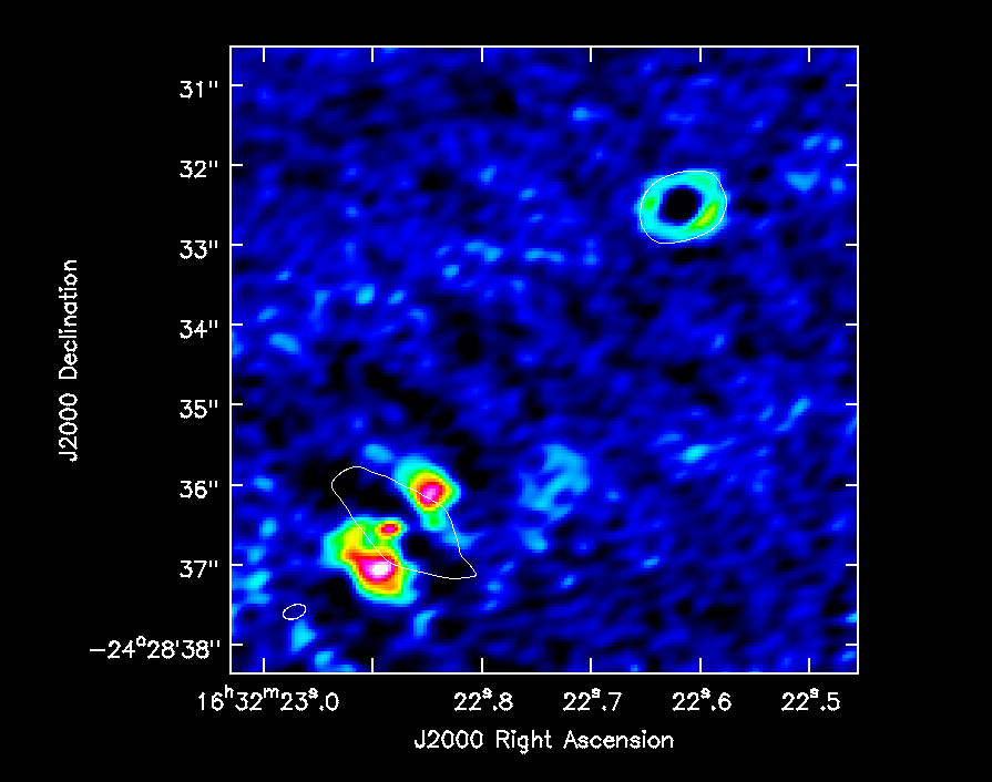
imview( raster=[ {'file':'IRAS16293_Band9.fixed.H13CN_8_7.image.subim.pbcor.mom0',
                 'range': [-1.,5.5]} ],
        contour={'file':'IRAS16293_Band9.fixed.CONTIN_AP.image.subim.pbcor',
                 'base':0, 'unit':0.025, 'levels':[3]},
        out='IRAS16293_Band9.fixed.H13CN_8_7.mom0.png')
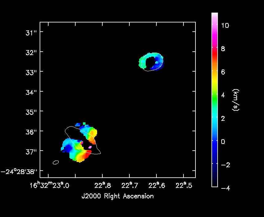
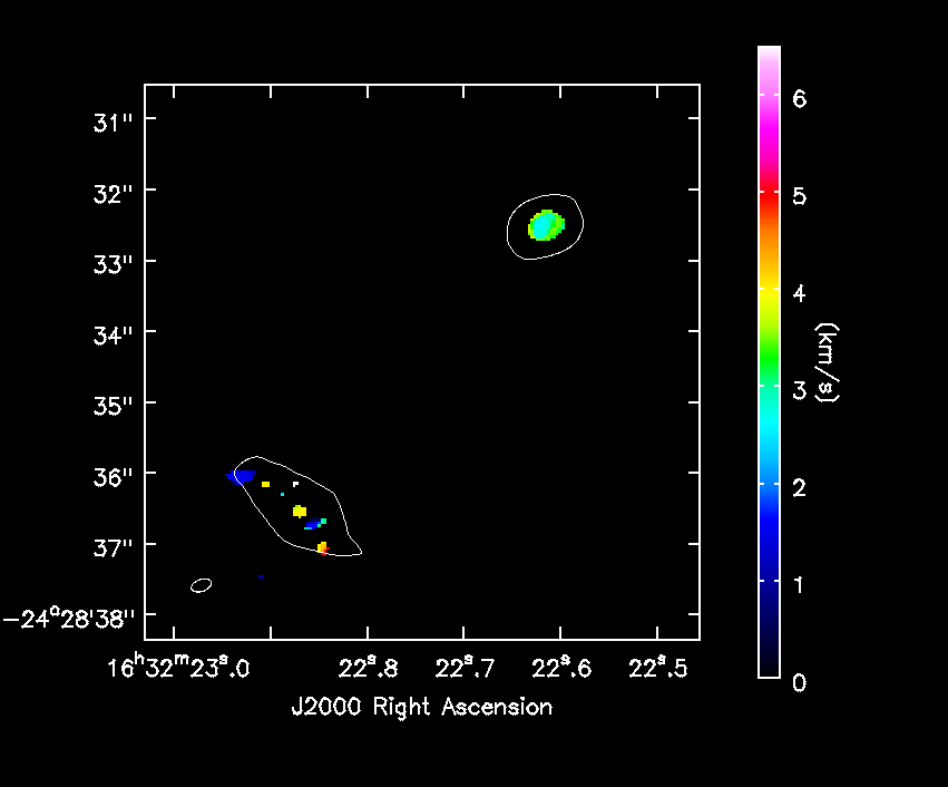
One cannot make higher order moments that simultaneously include both positive and negative emission. So we separate them below. Also, we need to restrict the higher order moments to regions of real signal. One way to do this is to use your clean mask to limit where we calculate the higherorder moments.
Next, we demonstrate how to use the clean mask for this purpose. We must first subimage it to match the primary beam corrected image. We also limit the pixels used to those with line emission greater than approximately 5sigma (5 times the rms noise value of the image):
immath(imagename='IRAS16293_Band9.fixed.H13CN_8_7.mask',
       mode='evalexpr',expr='IM0',box='221,160,493,430',
       outfile='IRAS16293_Band9.fixed.H13CN_8_7.mask.subim')
Producing the first and second moments in two steps, focusing first on the positive emission, and second on the negative (absorption) features:
os.system('rm -rf IRAS16293_Band9.fixed.H13CN_8_7.image.subim.pbcor.Positive*')
immoments(imagename='IRAS16293_Band9.fixed.H13CN_8_7.image.subim.pbcor',moments=[1,2],
          outfile='IRAS16293_Band9.fixed.H13CN_8_7.image.subim.pbcor.Positive',
          mask='IRAS16293_Band9.fixed.H13CN_8_7.mask.subim',
          chans='10~44',includepix=[0.4,100])

os.system('rm -rf IRAS16293_Band9.fixed.H13CN_8_7.image.subim.pbcor.Negative*')
immoments(imagename='IRAS16293_Band9.fixed.H13CN_8_7.image.subim.pbcor',moments=[1,2],
          outfile='IRAS16293_Band9.fixed.H13CN_8_7.image.subim.pbcor.Negative',
          mask='IRAS16293_Band9.fixed.H13CN_8_7.mask.subim',
          chans='10~44',includepix=[-100,-0.4])
Visualizing the maps:
imview( raster=[ {'file':'IRAS16293_Band9.fixed.H13CN_8_7.image.subim.pbcor.Negative.weighted_coord',
                 'colorwedge':True}],
        contour={'file':'IRAS16293_Band9.fixed.CONTIN_AP.image.subim.pbcor',
                 'base':0, 'unit':0.025, 'levels':[3]},
        out='IRAS16293_Band9.fixed.H13CN_8_7.Negative_mom1.png')
imview( raster=[ {'file':'IRAS16293_Band9.fixed.H13CN_8_7.image.subim.pbcor.Positive.weighted_coord',
                 'colorwedge':True}],
        contour={'file':'IRAS16293_Band9.fixed.CONTIN_AP.image.subim.pbcor',
                 'base':0, 'unit':0.025, 'levels':[3]},
        out='IRAS16293_Band9.fixed.H13CN_8_7.Positive_mom1.png')
And finally export the result to FITS format for further analysis:
os.system('rm -rf IRAS16293_Band9.fixed.H13CN_8_7.image.subim.pbcor.fits')
exportfits(imagename='IRAS16293_Band9.fixed.H13CN_8_7.image.subim.pbcor',
           fitsimage='IRAS16293_Band9.fixed.H13CN_8_7.image.subim.pbcor.fits')
os.system('rm -rf IRAS16293_Band9.fixed.H13CN_8_7.image.subim.pbcor.mom0.fits')
exportfits(imagename='IRAS16293_Band9.fixed.H13CN_8_7.image.subim.pbcor.mom0',
           fitsimage='IRAS16293_Band9.fixed.H13CN_8_7.image.subim.pbcor.mom0.fits')
os.system('rm -rf IRAS16293_Band9.fixed.H13CN_8_7.image.subim.pbcor.Negative.weighted_coord.fits')
exportfits(imagename='IRAS16293_Band9.fixed.H13CN_8_7.image.subim.pbcor.Negative.weighted_coord',
           fitsimage='IRAS16293_Band9.fixed.H13CN_8_7.image.subim.pbcor.Negative.weighted_coord.fits')
os.system('rm -rf IRAS16293_Band9.fixed.H13CN_8_7.image.subim.pbcor.Positive.weighted_coord.fits')
exportfits(imagename='IRAS16293_Band9.fixed.H13CN_8_7.image.subim.pbcor.Positive.weighted_coord',
           fitsimage='IRAS16293_Band9.fixed.H13CN_8_7.image.subim.pbcor.Positive.weighted_coord.fits')
os.system('rm -rf IRAS16293_Band9.fixed.H13CN_8_7.image.subim.pbcor.Negative.weighted_dispersion_coord.fits')
exportfits(imagename='IRAS16293_Band9.fixed.H13CN_8_7.image.subim.pbcor.Negative.weighted_dispersion_coord',
           fitsimage='IRAS16293_Band9.fixed.H13CN_8_7.image.subim.pbcor.Negative.weighted_dispersion_coord.fits')
os.system('rm -rf IRAS16293_Band9.fixed.H13CN_8_7.image.subim.pbcor.Positive.weighted_dispersion_coord.fits')
exportfits(imagename='IRAS16293_Band9.fixed.H13CN_8_7.image.subim.pbcor.Positive.weighted_dispersion_coord',
           fitsimage='IRAS16293_Band9.fixed.H13CN_8_7.image.subim.pbcor.Positive.weighted_dispersion_coord.fits')
Last checked on CASA Version 5.1.1.