Inspecting Data: Difference between revisions
No edit summary |
|||
| Line 24: | Line 24: | ||
Although the shadow and clip flags are plotted as well, the exact times affected by these flags are not known, so do not be alarmed by the fact that they appear to span the entire plot -- this is rarely actually the case. | Although the shadow and clip flags are plotted as well, the exact times affected by these flags are not known, so do not be alarmed by the fact that they appear to span the entire plot -- this is rarely actually the case. | ||
Unfortunately, since we requested time-averaged data from the archive, the flagged data are not included in the MS. If you are concerned about the possible erroneous deletion of good data, it's best to download the complete MS, inspect it with {{plotms}} (see below), and then perform time and / or frequency averaging. | Unfortunately, since we requested time-averaged data from the archive, the flagged data are not included in the MS. If you are concerned about the possible erroneous deletion of good data, it's best to download the complete MS, inspect it with {{plotms}} (see [[Inspecting_Data#Graphical_display:_plotms below]]), and then perform time and / or frequency averaging. | ||
== Checking the weather information == | == Checking the weather information == | ||
Revision as of 20:35, 20 April 2012
Overview
Now that you've obtained your measurement set (MS), you will probably want to look at it carefully to see what it contains. This CASA Guide will describe a set of CASA tasks designed to help you evaluate and understand the data in an MS.
Following the example in Loading Data, we will be using the MS TVER0002.sb2568947.eb2579996.55518.22356400463.ms in this Guide. Please see Loading Data for instructions on acquiring this dataset, or use your own MS for practice.
Checking the online flags

It's useful to start by checking which data have already been deleted (flagged) by the "online" flags (including time periods when the antennas were pointing off-source, or there were focus or subreflector errors), as well as data that were flagged because they were shadowed (blocked by a nearby antenna) or zero-valued (indicating a correlator error).
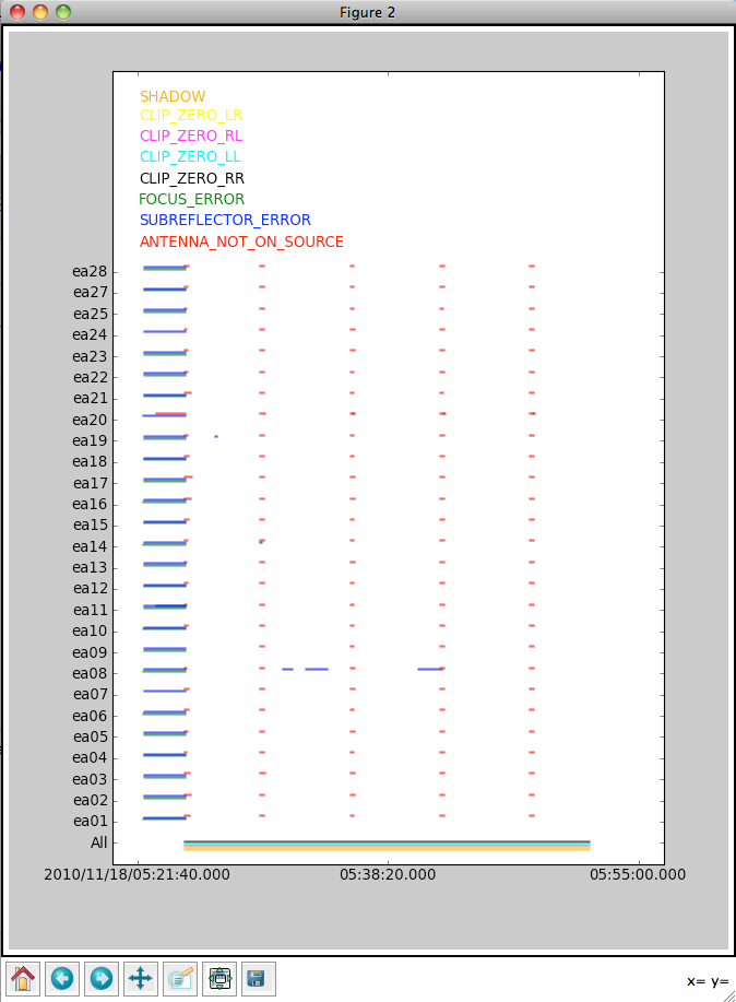
To do this, use the tflagcmd task to produce a plot:
# In CASA
tflagcmd(vis='TVER0002.sb2568947.eb2579996.55518.22356400463.ms',action='plot')
From this, we can see that antenna ea08 had some subreflector issues, and lengths of time when an antenna was not "on source" (i.e., it was slewing from one object to the next) varied a bit according to antenna. This accounts for the fact that the integration times provided by listobs are not exactly 10 s: the first integration of a given scan begins when the first antenna arrives on-source; since this does not happen simultaneously for all antennas, and the given integration time is an average across antennas, we can get values like 7.93 s (as for Scan 3).
Although the shadow and clip flags are plotted as well, the exact times affected by these flags are not known, so do not be alarmed by the fact that they appear to span the entire plot -- this is rarely actually the case.
Unfortunately, since we requested time-averaged data from the archive, the flagged data are not included in the MS. If you are concerned about the possible erroneous deletion of good data, it's best to download the complete MS, inspect it with plotms (see Inspecting_Data#Graphical_display:_plotms below), and then perform time and / or frequency averaging.