First Look at Self Calibration CASA 6.5.4: Difference between revisions
| (18 intermediate revisions by the same user not shown) | |||
| Line 1: | Line 1: | ||
==About this Guide== | ==About this Guide== | ||
{{checked_6.5.4}} | |||
{{CARTA_6.5.4}} | |||
This guide steps you through continuum imaging and self calibration | This guide steps you through continuum imaging and self calibration | ||
| Line 13: | Line 12: | ||
data, focusing on short-timescale phase corrections. | data, focusing on short-timescale phase corrections. | ||
First, copy the calibrated and flagged data from the working directory. Remember that this is our best version of the data. | First, copy the calibrated and flagged data from the working directory of the data tarball. Remember that this is our best version of the data. | ||
<source lang="python"> | <source lang="python"> | ||
| Line 35: | Line 34: | ||
For this and the other continuum first look tutorials, we have thus ignored the line to focus on the basic steps of imaging and self-calibration. | For this and the other continuum first look tutorials, we have thus ignored the line to focus on the basic steps of imaging and self-calibration. | ||
In general, however, you should flag channels containing emission lines in your own data prior to imaging the continuum. | In general, however, you should flag channels containing emission lines in your own data prior to imaging the continuum. | ||
To see how to flag line emission prior to imaging the continuum in a spectral window, please see the more advanced tutorial at [[ | To see how to flag line emission prior to imaging the continuum in a spectral window, please see the more advanced tutorial at [[IRAS16293Band9]]. | ||
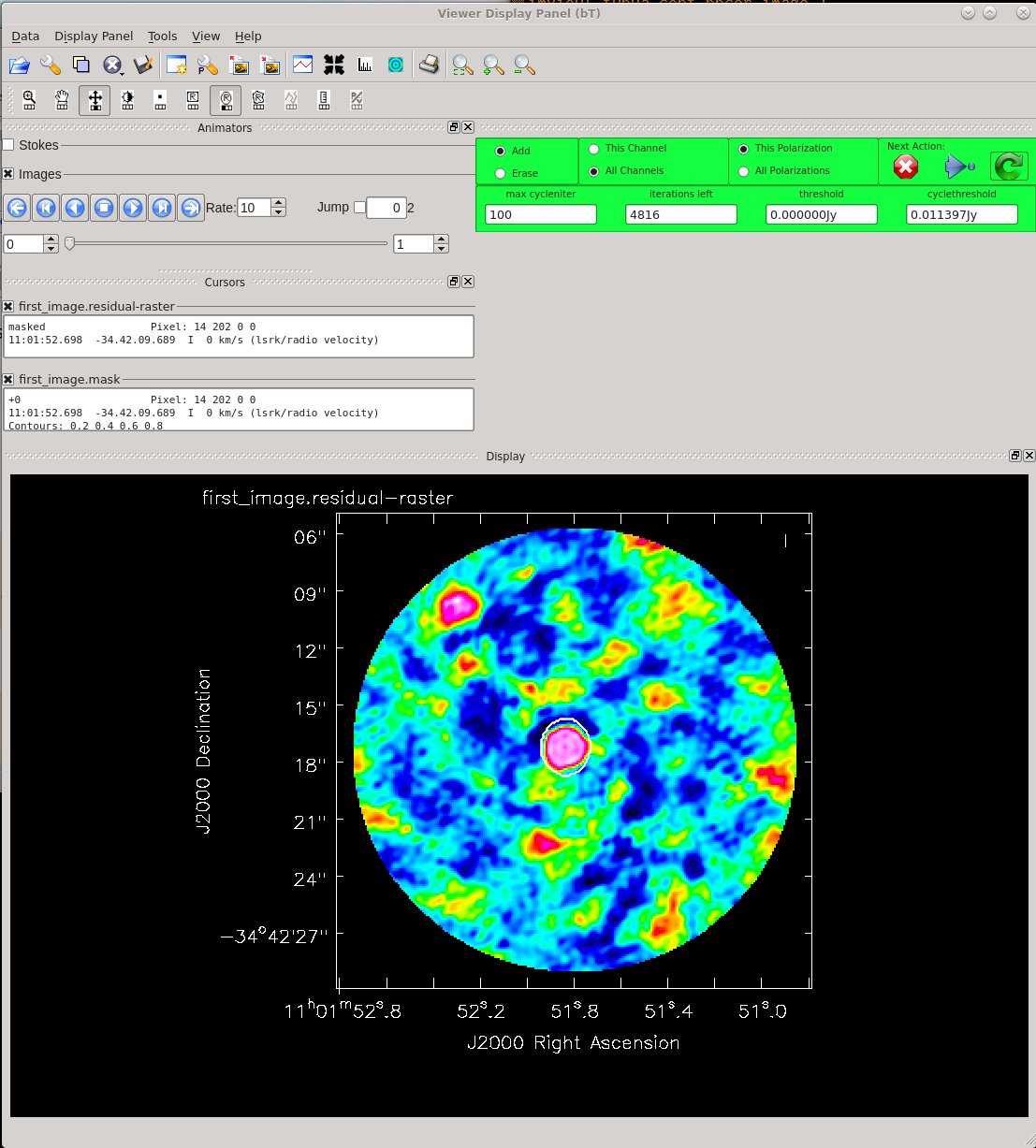
Clean until the residuals near TW Hydra are comparable | Clean until the residuals near TW Hydra are comparable | ||
to those in the rest of the image. For example, you might place your clean mask over the central feature, only, and clean with two major cycles. | to those in the rest of the image. For example, you might place your clean mask over the central feature, only, and clean with two major cycles. | ||
That is, use the green arrow twice, and then click the red X to finish tclean. '''Please note ''' that in general, it is good procedure to clean conservatively prior to the initial iterations of self-cal. Conservatively here means shallowly, erring on the side of missing some real flux instead of including flux that might be spurious. TW Hydra, being dominated by bright, compact emission, is relatively forgiving in that respect. For detailed discussion of these points see [[TWHydraBand7_Imaging_4.3#Create_Initial_Clean_Image | the TW Hydra CASA Guide]] and the self-calibration section of [[Self-Calibration_Template_CASA_6.5.4 | the guide to the NA Imaging Template Script]]. | That is, use the green arrow twice, and then click the red X to finish tclean. '''Please note ''' that in general, it is good procedure to clean conservatively prior to the initial iterations of self-cal. Conservatively here means shallowly, erring on the side of missing some real flux instead of including flux that might be spurious. TW Hydra, being dominated by bright, compact emission, is relatively forgiving in that respect. For detailed discussion of these points see [[TWHydraBand7_Imaging_4.3#Create_Initial_Clean_Image | the TW Hydra CASA Guide]] and the self-calibration section of [[Self-Calibration_Template_CASA_6.5.4 | the guide to the NA Imaging Template Script]]. | ||
[[File:Imaging-tutorial-selfcal-1_6.5.4.jpeg|thumb|<caption>Figure 1: Residuals from the first tclean after final cycle of cleaning. | [[File:Imaging-tutorial-selfcal-1_6.5.4.jpeg|thumb|<caption>Figure 1: Residuals from the first tclean after final cycle of cleaning. | ||
Image Statistics: Beam 0.560", 0.416", -55.974°, RMS = 6.6 mJy </caption>]] | Image Statistics: Beam 0.560", 0.416", -55.974°, RMS = 6.6 mJy </caption>]] | ||
<source lang="python"> | <source lang="python"> | ||
| Line 65: | Line 62: | ||
savemodel='modelcolumn') | savemodel='modelcolumn') | ||
</source> | </source> | ||
In addition to creating an image, TCLEAN saves the cleaned "model" of the science target with | In addition to creating an image, TCLEAN saves the cleaned "model" of the science target with | ||
| Line 123: | Line 119: | ||
is to have no failed solutions at all, and to have good S/N on the solutions we do get. (Always S/N > 3, but ideally | is to have no failed solutions at all, and to have good S/N on the solutions we do get. (Always S/N > 3, but ideally | ||
S/N>5 or better.) | S/N>5 or better.) | ||
Try playing around with different solution intervals or averaging | Try playing around with different solution intervals or averaging | ||
| Line 149: | Line 143: | ||
tracking one another pretty well. If the data were already perfectly | tracking one another pretty well. If the data were already perfectly | ||
calibrated, these values would solve to be zero. | calibrated, these values would solve to be zero. | ||
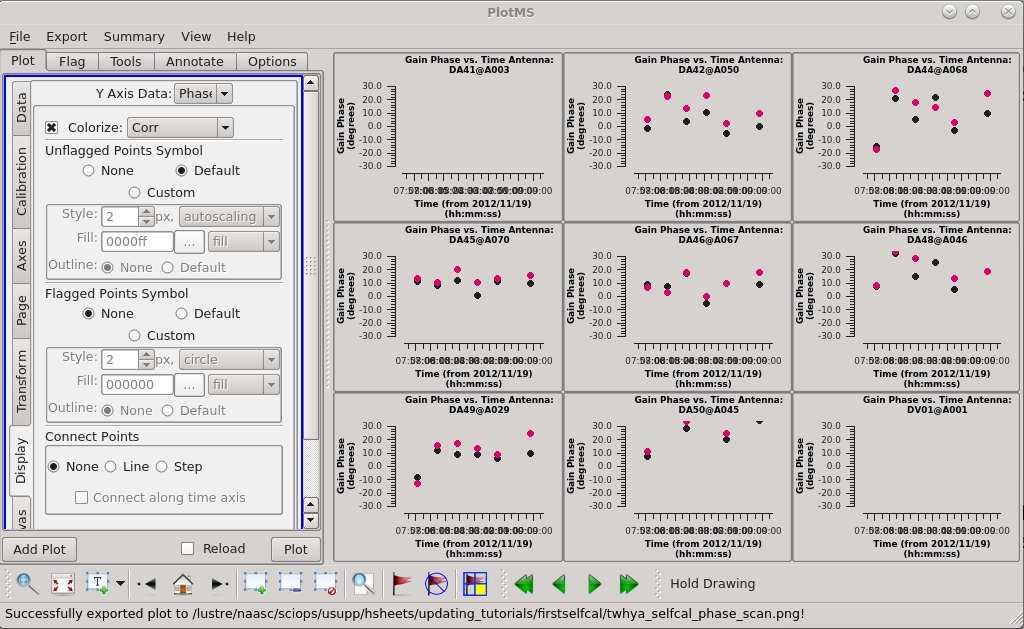
[[File:Imaging-tutorial-selfcal-plotcal-1_6.5.4.jpg|thumb|<caption>Figure 2: Phase solutions after the first round of self calibration.</caption>]] | [[File:Imaging-tutorial-selfcal-plotcal-1_6.5.4.jpg|thumb|<caption>Figure 2: Phase solutions after the first round of self calibration.</caption>]] | ||
<source lang="python"> | <source lang="python"> | ||
| Line 179: | Line 171: | ||
applycal(vis='twhya_calibrated.ms', | applycal(vis='twhya_calibrated.ms', | ||
field='5', | field='5', | ||
gaintable=[phase.cal], | gaintable=['phase.cal'], | ||
interp='linear') | interp='linear') | ||
</source> | </source> | ||
| Line 200: | Line 192: | ||
Now clean the self-calibrated data. Again, clean until the residuals | Now clean the self-calibrated data. Again, clean until the residuals | ||
on TW Hydra resemble those in the surrounding image. We can clean a little deeper this time. | on TW Hydra resemble those in the surrounding image. We can clean a little deeper this time. | ||
[[File:Imaging-tutorial-selfcal-2_6.5.4.jpg|thumb|<caption>Figure 3: Residuals from the second tclean after 5 major cycles of cleaning. </caption>]] | [[File:Imaging-tutorial-selfcal-2_6.5.4.jpg|thumb|<caption>Figure 3: Residuals from the second tclean after 5 major cycles of cleaning. </caption>]] | ||
<source lang="python"> | <source lang="python"> | ||
| Line 228: | Line 218: | ||
The residuals do look better this time around. Use CARTA to | The residuals do look better this time around. Use CARTA to | ||
compare the first and second images. You should see a noticeable | compare the first and second images. If you are using NRAO machines, you can navigate to your working directory in a terminal, and then type: | ||
<source lang="bash"> | |||
# In bash | |||
carta --no_browser | |||
</source> | |||
[[File:Imaging-tutorial-selfcal-comp_6.5.4.jpg|thumb|<caption>Figure 4: Side by side view of first_image.image and second_image.image in CARTA. Matching the raster scaling between the two images shows the improvement generally in the RMS. Define a region and open the statistics widget to find the average RMS within the region.</caption>]] | |||
Copy the URL it returns and paste into a browser window to view your CARTA session. Load the first image and then "append" the second image to bring up both (or ctrl+click in the "Open Image" dialog box to select the second image along with the first). Create a region using the rectangle, ellipse, or polygon tool at the top. You can save the region using "Export Regions" from the "File" menu and load it on the second image, if you like, using "Import Regions". Then click the button at the top that looks like a calculator to view the statistics. You should see a noticeable | |||
improvement in the noise and some improvement in the signal, so that | improvement in the noise and some improvement in the signal, so that | ||
the overall signal-to-noise (dynamic range) is much improved. | the overall signal-to-noise (dynamic range) is much improved. If you match the raster scaling between images (by clicking the R in the Matching column for the second image in the Image List at the lower right of the CARTA window), you can also see that the noise is much more uniform in the second (i.e. post self-cal) image. (To view the images side by side, as in Figure 4, click the "switch to multipanel" button just above the panel displaying the image in CARTA - it looks like a square.) | ||
This second clean also produces a model (if the savemodel parameter is set!), hopefully a mildly better one this time. | This second clean also produces a model (if the savemodel parameter is set!), hopefully a mildly better one this time. | ||
| Line 258: | Line 255: | ||
do much. | do much. | ||
[[File:Imaging-tutorial-selfcal-plotcal-2_6.5.4.jpg|thumb|<caption>Figure 5: Phase solutions after the second round of self calibration.</caption>]] | |||
[[File:Imaging-tutorial-selfcal-plotcal-2_6.5.4.jpg|thumb|<caption>Figure | |||
<source lang="python"> | <source lang="python"> | ||
| Line 271: | Line 266: | ||
iteraxis='antenna', | iteraxis='antenna', | ||
plotrange=[0,0,-30,30], | plotrange=[0,0,-30,30], | ||
coloraxis= | coloraxis='corr', | ||
titlefont=7, | titlefont=7, | ||
xaxisfont=7, | xaxisfont=7, | ||
| Line 305: | Line 300: | ||
Clean a third time. | Clean a third time. | ||
[[File:Imaging-tutorial-selfcal-3_6.5.4.jpg|thumb|<caption>Figure | [[File:Imaging-tutorial-selfcal-3_6.5.4.jpg|thumb|<caption>Figure 6: Residuals from the third clean after 6 main cycles of cleaning. </caption>]] | ||
<source lang="python"> | <source lang="python"> | ||
| Line 353: | Line 348: | ||
iteraxis='antenna', | iteraxis='antenna', | ||
plotrange=[0,0,-30,30], | plotrange=[0,0,-30,30], | ||
coloraxis= | coloraxis='corr', | ||
titlefont=7, | titlefont=7, | ||
xaxisfont=7, | xaxisfont=7, | ||
| Line 361: | Line 356: | ||
</source> | </source> | ||
[[File:Imaging-tutorial-selfcal-plotcal-3_6.5.4.jpg|thumb|<caption>Figure | [[File:Imaging-tutorial-selfcal-plotcal-3_6.5.4.jpg|thumb|<caption>Figure 7: Phase solutions after the third round of self calibration. </caption>]] | ||
==Apply the Third Phase Calibration== | ==Apply the Third Phase Calibration== | ||
| Line 408: | Line 403: | ||
savemodel='modelcolumn') | savemodel='modelcolumn') | ||
</source> | </source> | ||
[[File:Imaging-tutorial-selfcal-image-4_6.5.4.jpg|thumb|<caption>Figure | [[File:Imaging-tutorial-selfcal-image-4_6.5.4.jpg|thumb|<caption>Figure 8: Residuals from the fourth clean after 7 major cycles of cleaning. </caption>]] | ||
| Line 420: | Line 415: | ||
<source lang="python"> | <source lang="python"> | ||
# In CASA | |||
os.system('rm -rf amp.cal') | os.system('rm -rf amp.cal') | ||
gaincal(vis='twhya_selfcal_3.ms', | gaincal(vis='twhya_selfcal_3.ms', | ||
| Line 440: | Line 436: | ||
<source lang="python"> | <source lang="python"> | ||
# In CASA | |||
plotms(vis='amp.cal', | plotms(vis='amp.cal', | ||
xaxis='time', | xaxis='time', | ||
| Line 457: | Line 454: | ||
</source> | </source> | ||
[[File:Imaging-tutorial-selfcal-plotcal-4_6.5.4.jpg|thumb|<caption>Figure | [[File:Imaging-tutorial-selfcal-plotcal-4_6.5.4.jpg|thumb|<caption>Figure 9: Phase solutions after the fourth round of self calibration. </caption>]] | ||
We see a good deal of scatter and some offsets between | We see a good deal of scatter and some offsets between | ||
correlations. This can be easily visualized within the plotms viewer by selecting the "Display" tab, checking the "colorize" box, and selecting "corr" to colorize the data by correlation. It is at least worth looking at what the effects of applying this will be. So let's apply these solutions. | correlations. This can be easily visualized within the plotms viewer by selecting the "Display" tab, checking the "colorize" box, and selecting "corr" to colorize the data by correlation. It is at least worth looking at what the effects of applying this will be. So let's apply these solutions. | ||
<source lang="python"> | <source lang="python"> | ||
# In CASA | |||
applycal(vis='twhya_selfcal_3.ms', | applycal(vis='twhya_selfcal_3.ms', | ||
field='5', | field='5', | ||
| Line 472: | Line 469: | ||
At this point the self-calibrated data live in the corrected | At this point the self-calibrated data live in the corrected | ||
column. Let's split out the corrected data once again, to preserve this calibration. | column. Let's split out the corrected data once again, to preserve this calibration. | ||
<source lang="python"> | <source lang="python"> | ||
# In CASA | |||
os.system('rm -rf twhya_selfcal4.ms*') | os.system('rm -rf twhya_selfcal4.ms*') | ||
split(vis='twhya_selfcal_3.ms', | |||
outputvis='twhya_selfcal_4.ms', | outputvis='twhya_selfcal_4.ms', | ||
datacolumn='corrected') | datacolumn='corrected') | ||
| Line 483: | Line 480: | ||
Clean a fifth time to view our results. Since we don't plan to do another round of calibration, no need to use savemodel='modelcolumn' here. | Clean a fifth time to view our results. Since we don't plan to do another round of calibration, no need to use savemodel='modelcolumn' here. | ||
[[File:Imaging-tutorial-selfcal-4_6.5.4.jpg|thumb|<caption>Figure | [[File:Imaging-tutorial-selfcal-4_6.5.4.jpg|thumb|<caption>Figure 10: Residuals from the fifth tclean after 8 major cycles of cleaning. </caption>]] | ||
<source lang="python"> | <source lang="python"> | ||
# In CASA | |||
os.system('rm -rf fifth_image.*') | os.system('rm -rf fifth_image.*') | ||
tclean(vis='twhya_selfcal_4.ms', | tclean(vis='twhya_selfcal_4.ms', | ||
| Line 503: | Line 501: | ||
</source> | </source> | ||
Image Statistics: Beam | Image Statistics: Beam 0.598", 0.446", -54.912°, RMS = 2.0 mJy | ||
This time, notice from the residuals that you can clean more deeply. After 4 main cycles, the background residuals look very random on | This time, notice from the residuals that you can clean more deeply. After 4 main cycles, the background residuals look very random on | ||
Latest revision as of 18:53, 5 August 2024
About this Guide
Last checked on CASA Version 6.5.4
This guide features CARTA, the “Cube Analysis and Rendering Tool for Astronomy,” which is the new NRAO visualization tool for images and cubes. The CASA viewer (imview) has not been maintained for a few years and will be removed from future versions of CASA. We strongly recommend using CARTA, as it provides a much more efficient, stable, and feature rich user experience. A comparison of the CASA viewer and CARTA, as well as instructions on how to use CARTA at NRAO, is provided in the CARTA section of the CASA docs.
This guide steps you through continuum imaging and self calibration of the science data for our science target, TW Hydra.
Getting the Data
You should have downloaded the data package as part of the previous imaging tutorial. If you haven't done that yet, check the First_Look_at_Imaging_CASA_6.5.4 Guide for instructions.
In the previous tutorial, you made a first continuum image. We start here by repeating that step, and then we iteratively self-calibrate the data, focusing on short-timescale phase corrections.
First, copy the calibrated and flagged data from the working directory of the data tarball. Remember that this is our best version of the data.
# In CASA
os.system('rm -rf twhya_calibrated.ms')
os.system('tar -xvf ../working/twhya_calibrated.ms.tar')
Run a quick listobs to get oriented:
# In CASA
listobs('twhya_calibrated.ms')
Creating a Model for Self Calibration in tclean
Now, use tclean to make a continuum image of TW Hydra (field 5). This call is interactive, but the automated approach that we used in the last lesson would also work. See the last lesson for details. Remember that the spectral window that we will image here as continuum also contains a N2H+ emission line. In this case, the N2H+ emission is faint enough that neglecting to flag the line channels before imaging makes no difference to the final continuum image. For this and the other continuum first look tutorials, we have thus ignored the line to focus on the basic steps of imaging and self-calibration. In general, however, you should flag channels containing emission lines in your own data prior to imaging the continuum. To see how to flag line emission prior to imaging the continuum in a spectral window, please see the more advanced tutorial at IRAS16293Band9.
Clean until the residuals near TW Hydra are comparable to those in the rest of the image. For example, you might place your clean mask over the central feature, only, and clean with two major cycles. That is, use the green arrow twice, and then click the red X to finish tclean. Please note that in general, it is good procedure to clean conservatively prior to the initial iterations of self-cal. Conservatively here means shallowly, erring on the side of missing some real flux instead of including flux that might be spurious. TW Hydra, being dominated by bright, compact emission, is relatively forgiving in that respect. For detailed discussion of these points see the TW Hydra CASA Guide and the self-calibration section of the guide to the NA Imaging Template Script.
# In CASA
os.system('rm -rf first_image.*')
tclean(vis='twhya_calibrated.ms',
       imagename='first_image',
       field='5',
       spw='',
       specmode='mfs',
       deconvolver='hogbom',
       nterms=1,
       gridder='standard',
       imsize=[250,250],
       cell=['0.1arcsec'],
       weighting='briggs',
       threshold='0mJy',
       niter=5000,
       interactive=True,
       savemodel='modelcolumn')
In addition to creating an image, TCLEAN saves the cleaned "model" of the science target with the measurement set if the parameter savemodel="modelcolumn". This model is required for later self-calibration steps. Of course this model for our science target is not perfect; It's only as good as the first clean, but it's a good starting point. Look for the line in the log that says 'Saving model column' to be sure that the model has been saved.
Creating the First Phase Calibration Table
With a model in place, we are in a position to calibrate the science target directly. We use gaincal, which is the task used both for general gain calibration using an external calibrator, and for self-calibration. We will focus here on phase corrections - generally good practice for self calibration - because amplitude self calibration has a larger potential to change the source characteristics (i.e. introduce artifacts). Figuring out the best averaging parameters is often the key to good self-calibration. You would like the solution interval to be short enough so that it tracks changes in the atmospheric phase with high accuracy, but long enough so that you measure phases with good signal-to-noise. Also, ideally you'd like to keep solutions separate for difference spw's and polarizations, but for faint sources when you need to boost SNR, it may be necessary to average over these parameters to achieve good solutions. Using 30 seconds for the solution interval turns out to be a good choice for TW Hydra, but we'll start with the longest solution, solint='inf' (i.e. the full length of a scan).
# In CASA
os.system('rm -rf phase.cal')
gaincal(vis='twhya_calibrated.ms',
        caltable='phase.cal',
        field='5',
        solint='inf',
        calmode='p',
        refant='DV22',
        gaintype='G')
Gaincal does the following: it looks at your ‘data’ column, looks at your ‘model’ column, and figures out what correction needs to be applied to ‘data’ in order to make it look like ‘model.’ It produces a calibration table (‘*.cal’ file) with these corrections for each antenna and time, but it does not actually apply these corrections. Applying the corrections is done with the applycal task (see below).
Figuring out the best averaging parameters is often the key to good self-calibration. You would like the solution interval to be short enough so that it tracks changes in the atmospheric phase with high accuracy, but long enough so that you measure phases with good signal-to-noise. Also, ideally you’d like to keep solutions separate for different spws and polarizations. For faint sources when you need to boost SNR, however, it may be necessary to average over these parameters to achieve good solutions.
Solint Values: In gaincal, the parameter ’solint’ determines the time interval over which gaincal will derive phase solutions. Ideally this should be an integer multiple of your integration time (i.e. if your integration time is 3s, your solint values might be solint=3s, solint=6s, solint=9s, etc.). Solint can range from ‘int’ at minimum (i.e., ‘integration,’ your integration time for a single integration) to ‘inf’ at maximum (i.e. ‘infinity,’ which is not actually infinity but rather the maximum time interval allowed.). If you have combine=‘’ set, setting ‘inf’ will be equivalent to combining all integrations within a single scan, but will not combine across scans (i.e. if your integration time is 3s, and each scan was 2 minutes long, setting solint=‘inf’ is equivalent to setting solint=‘120s’). If you set combine=‘scan,’ the effective value of solint=‘inf’ will likewise increase.
Gaintype: ‘gaintype’=‘G’ will cause gaincal to derive solutions for each polarization independently. This becomes more important if you have a polarized source or a source whose polarization state you do not know. If your source is unpolarized, it is still a good idea to use ‘gaintype=G’ if you can, as this will yield the most accurate solutions. However, if you need to increase the S/N of your solutions, ‘calmode’=‘T’ will combine the data across polarizations and derive a single solution for both.
In the gaincal example above, the first choice of solint is entirely arbitrary. Try it and see what you get. Our goal is to have no failed solutions at all, and to have good S/N on the solutions we do get. (Always S/N > 3, but ideally S/N>5 or better.)
Try playing around with different solution intervals or averaging options. Bear in mind that you want the shortest possible interval while also retaining separate SPW and polarizations. However, none of this helps you if you don't get good solutions. So you generally will experiment with the following options: (1) combine="scan" or "spw" to allow solutions to cross SPW/scan boundaries, or you can do both using combine="scan,spw"; (2) increase solint to set the solution interval; and (3) toggling gaintype between "G" and "T" (the former generates solutions independently for each polarization, and the latter averages two polarizations before determining the solutions).
It maybe helpful to graph the signal-to-noise ratio (SNR) vs. time or the phase vs. time for different settings using plotms. Note the differences in the SNR for different solint values.
# In CASA
plotms(vis='phase.cal', xaxis='time', yaxis='SNR')
# In CASA
plotms(vis='phase.cal', xaxis='time', yaxis='phase')
Plot the resulting solutions. We are finding nontrivial, though not enormous, solutions (a few 10s of degrees) with the two correlations tracking one another pretty well. If the data were already perfectly calibrated, these values would solve to be zero.
# In CASA
plotms(vis='phase.cal',
       xaxis='time',
       yaxis='phase',
       gridrows=3,
       gridcols=3,
       iteraxis='antenna',
       plotrange=[0,0,-30,30],
       coloraxis='corr',
       titlefont=7,
       xaxisfont=7,
       yaxisfont=7,
       plotfile='twhya_selfcal_phase_scan.png',
       showgui = True)
Apply the First Phase Calibration
We are happy with this solution. So let's apply it to the data using applycal. We only care about field 5 (the science target).
# In CASA
applycal(vis='twhya_calibrated.ms',
         field='5',
         gaintable=['phase.cal'],
         interp='linear')
At this point the self-calibrated data are stored in the MS in the "corrected data" column. Because we will want to try more rounds of self calibration, it's often useful (though not strictly necessary) at this point to split out the corrected data into a new data set. If you are restarting this tutorial, you need to first delete the output .ms and .flagversions file.
# In CASA
os.system('rm -rf twhya_selfcal.ms twhya_selfcal.ms.flagversions')
split(vis='twhya_calibrated.ms',
      outputvis='twhya_selfcal.ms',
      datacolumn='corrected')
Create an Improved Model
Now clean the self-calibrated data. Again, clean until the residuals on TW Hydra resemble those in the surrounding image. We can clean a little deeper this time.

# In CASA
os.system('rm -rf second_image.*')
tclean(vis='twhya_selfcal.ms',
       imagename='second_image',
       field='5',
       spw='',
       specmode='mfs',
       deconvolver='hogbom',
       nterms=1,
       gridder='standard',
       imsize=[250,250],
       cell=['0.1arcsec'],
       weighting='briggs',
       threshold='0mJy',
       interactive=True,
       niter=5000,
       savemodel='modelcolumn')
Image Statistics: Beam 0.559", 0.415", -55.877°, RMS = 2.4 mJy
The residuals do look better this time around. Use CARTA to compare the first and second images. If you are using NRAO machines, you can navigate to your working directory in a terminal, and then type:
# In bash
carta --no_browser
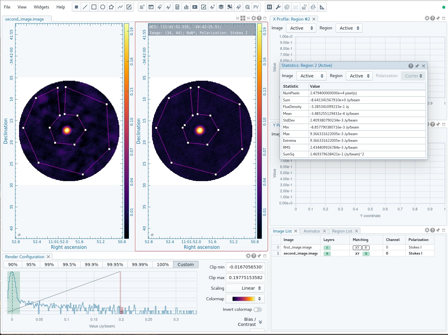
Copy the URL it returns and paste into a browser window to view your CARTA session. Load the first image and then "append" the second image to bring up both (or ctrl+click in the "Open Image" dialog box to select the second image along with the first). Create a region using the rectangle, ellipse, or polygon tool at the top. You can save the region using "Export Regions" from the "File" menu and load it on the second image, if you like, using "Import Regions". Then click the button at the top that looks like a calculator to view the statistics. You should see a noticeable improvement in the noise and some improvement in the signal, so that the overall signal-to-noise (dynamic range) is much improved. If you match the raster scaling between images (by clicking the R in the Matching column for the second image in the Image List at the lower right of the CARTA window), you can also see that the noise is much more uniform in the second (i.e. post self-cal) image. (To view the images side by side, as in Figure 4, click the "switch to multipanel" button just above the panel displaying the image in CARTA - it looks like a square.)
This second clean also produces a model (if the savemodel parameter is set!), hopefully a mildly better one this time.
Create Second Phase Calibration Table
Now we will run a second round of phase-only self calibration using the improved model and a shorter time interval (solint).
# In CASA
os.system('rm -rf phase_2.cal')
gaincal(vis='twhya_selfcal.ms',
        caltable='phase_2.cal',
        field='5',
        solint='170s',
        calmode='p',
        refant='DV22',
        gaintype='G')
This time we see a number of failed solutions that gaincal has flagged due to insufficient signal to noise (compared to the threshold set by minSNR). A small number of failed solutions may be expected depending on the solution interval, especially for more extended antennas in the configuration, although ideally you will find a solint that gives you no failed solutions. Failed solutions mean that those data will get flagged (i.e. no longer used) automatically. It is important to take into account how the resultant flagged baselines affect the beam size and image fidelity after each gaincal iteration.
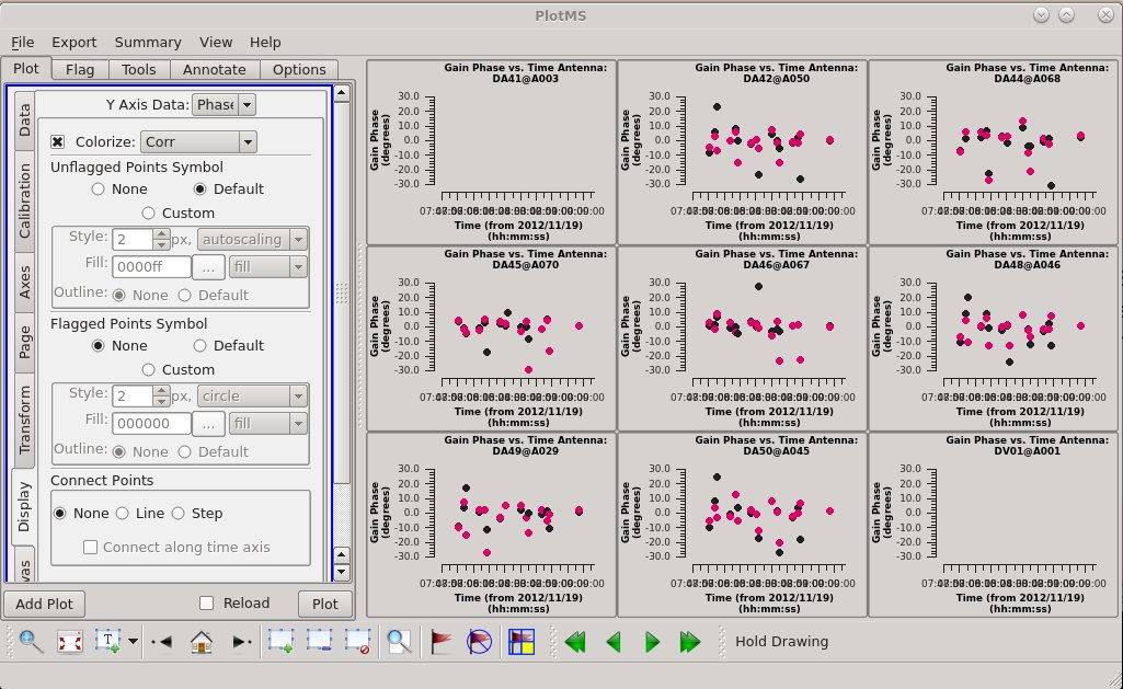
Let's plot the calibration table again. At this point, we see much smaller phase scatter relative to the model, so we don't expect more phase-only self calibration to do much.
# In CASA
plotms(vis='phase_2.cal',
       xaxis='time',
       yaxis='phase',
       gridrows=3,
       gridcols=3,
       iteraxis='antenna',
       plotrange=[0,0,-30,30],
       coloraxis='corr',
       titlefont=7,
       xaxisfont=7,
       yaxisfont=7,
       plotfile='twhya_selfcal_phase_scan_2.png',
       showgui = True)
Apply the Second Phase Calibration
Apply the solutions again:
# In CASA
applycal(vis='twhya_selfcal.ms',
         field='5',
         gaintable=['phase_2.cal'],
         interp='linear')
Split the data off again. Here you can see the work flow for heavily iterative self-calibration. We progressively calibrate, split.
# In CASA
os.system('rm -rf twhya_selfcal_2.ms twhya_selfcal_2.ms.flagversions')
split(vis='twhya_selfcal.ms',
      outputvis='twhya_selfcal_2.ms',
      datacolumn='corrected')
Improve the Model Further
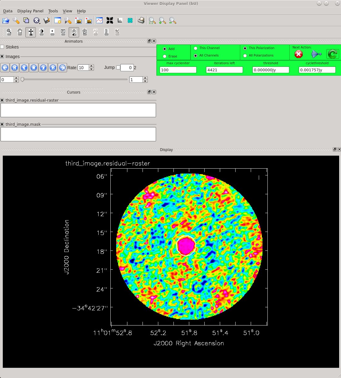
Clean a third time.
# In CASA
os.system('rm -rf third_image.*')
tclean(vis='twhya_selfcal_2.ms',
       imagename='third_image',
       field='5',
       spw='',
       specmode='mfs',
       deconvolver='hogbom',
       nterms=1,
       gridder='standard',
       imsize=[250,250],
       cell=['0.1arcsec'],
       weighting='briggs',
       threshold='0mJy',
       interactive=True,
       niter=5000,
       savemodel='modelcolumn')
Image Statistics: Beam 0.580", 0.439", -57.771°, RMS = 2.3 mJy
Create the Third Phase Calibration Table
Run a third round of phase-only self calibration using the improved model and a still-shorter time interval (solint).
# In CASA
os.system('rm -rf phase_3.cal')
gaincal(vis='twhya_selfcal_2.ms',
        caltable='phase_3.cal',
        field='5',
        solint='30s',
        calmode='p',
        refant='DV22',
        gaintype='T')
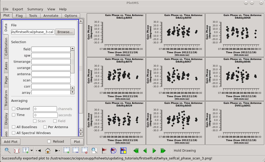
# Plot the amplitude solutions.
plotms(vis='phase_3.cal',
       xaxis='time',
       yaxis='phase',
       gridrows=3,
       gridcols=3,
       iteraxis='antenna',
       plotrange=[0,0,-30,30],
       coloraxis='corr',
       titlefont=7,
       xaxisfont=7,
       yaxisfont=7,
       plotfile='twhya_selfcal_phase_scan_3.png',
       showgui = True)
Apply the Third Phase Calibration
Apply the solutions again:
# In CASA
applycal(vis='twhya_selfcal_2.ms',
         field='5',
         gaintable=['phase_3.cal'],
         interp='linear')
Split the data off again:
# In CASA
os.system('rm -rf twhya_selfcal_3.ms twhya_selfcal_3.ms.flagversions')
split(vis='twhya_selfcal_2.ms',
      outputvis='twhya_selfcal_3.ms',
      datacolumn='corrected')
Improve the Model Again
Clean for a fourth time. Remember to set savemodel='modelcolumn' if you want to continue iterating on the self-calibration.
# In CASA
os.system('rm -rf fourth_image.*')
tclean(vis='twhya_selfcal_3.ms',
       imagename='fourth_image',
       field='5',
       spw='',
       specmode='mfs',
       deconvolver='hogbom',
       nterms=1,
       gridder='standard',
       imsize=[250,250],
       cell=['0.1arcsec'],
       weighting='briggs',
       threshold='0mJy',
       interactive=True,
       niter=5000,
       savemodel='modelcolumn')
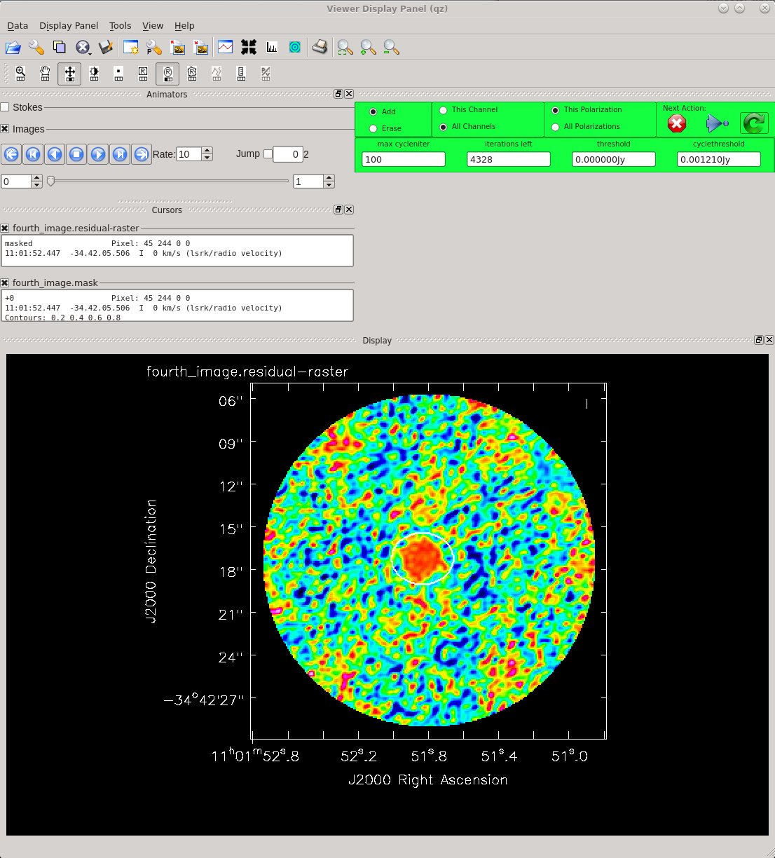
Image Statistics: Beam 0.599", 0.444", -54.643°, RMS = 2.1 mJy
Amplitude Self Calibration
In many cases, it would be perfectly fine to stop self-calibrating once we are satisfied with our phase-only self-calibration solutions. In this case, however, we will move on to demonstrating amplitude+phase self-cal. This type of self-cal is potentially dangerous as it has much more potential to change the characteristics of the source than phase self-calibration. We mitigate this somewhat by setting solnorm=True, so that the solutions are normalized.
# In CASA
os.system('rm -rf amp.cal')
gaincal(vis='twhya_selfcal_3.ms',
        caltable='amp.cal',
        field='5',
        solint='inf',
        calmode='ap',
        refant='DV22',
        gaintype='G',
        gaintable=['phase_3.cal'],
        solnorm=True)
Note that we have increased our solint back to ’inf.’ This is common for amplitude self-cal: you will want a solint for the amplitude self-cal that is larger than the solint for your best round of phase-only self-cal. We have also added the line ’gaintable=...’ This is because we don’t want to let ap self-cal have too many degrees of freedom. Instead, we force it to use our phase-only solutions first, before it is allowed to calculate amplitude+phase solutions.
Plot the calibration table again:
# In CASA
plotms(vis='amp.cal',
       xaxis='time',
       yaxis='amp',
       gridrows=3,
       gridcols=3,
       iteraxis='antenna',
       plotrange=[0,0,0,0],
       coloraxis='corr',
       titlefont=7,
       xaxisfont=7,
       yaxisfont=7,
       plotfile='twhya_selfcal_amp_scan.png',
       showgui = True)
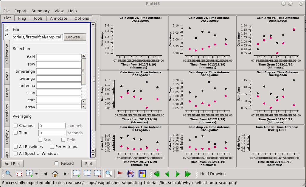
We see a good deal of scatter and some offsets between correlations. This can be easily visualized within the plotms viewer by selecting the "Display" tab, checking the "colorize" box, and selecting "corr" to colorize the data by correlation. It is at least worth looking at what the effects of applying this will be. So let's apply these solutions.
# In CASA
applycal(vis='twhya_selfcal_3.ms',
         field='5',
         gaintable=['phase_3.cal','amp.cal'],
         interp='linear')
At this point the self-calibrated data live in the corrected column. Let's split out the corrected data once again, to preserve this calibration.
# In CASA
os.system('rm -rf twhya_selfcal4.ms*')
split(vis='twhya_selfcal_3.ms',
      outputvis='twhya_selfcal_4.ms',
      datacolumn='corrected')
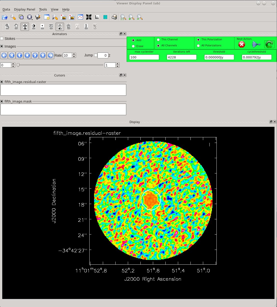
Clean a fifth time to view our results. Since we don't plan to do another round of calibration, no need to use savemodel='modelcolumn' here.
# In CASA
os.system('rm -rf fifth_image.*')
tclean(vis='twhya_selfcal_4.ms',
       imagename='fifth_image',
       field='5',
       spw='',
       specmode='mfs',
       deconvolver='hogbom',
       nterms=1,
       gridder='standard',
       imsize=[250,250],
       cell=['0.1arcsec'],
       weighting='briggs',
       threshold='0mJy',
       interactive=True,
       niter=5000)
Image Statistics: Beam 0.598", 0.446", -54.912°, RMS = 2.0 mJy
This time, notice from the residuals that you can clean more deeply. After 4 main cycles, the background residuals look very random on the scale of the beam size. This is good!
Compare the fourth and fifth images (you can use an imstat command or inspect the images in CARTA). The noise level is better, while the flux has not changed markedly (this is very good, it's what we worry about with amplitude self calibration).
By assuming that the previous cleans represent good models we have managed to improve the signal-to-noise on the data by over a factor of 3. Not bad!
Whether you are satisfied with the apcal self-calibration in this case or not, it is very important to understand that amplitude+phase self-cal is not always successful, nor is it always necessary. If you can get good solutions with apcal self-calibration, you will likely have improved your S/N ratio by an order of magnitude or more over the non-self- calibrated data. Likewise, if you have had a significant improvement with phase-only self-cal, and you can’t get good solutions for amplitude+phase, that’s okay - you have still significantly improved your data!
In this case the fifth image is our best continuum image. We can use the data set (twhya_selfcal_4.ms) to proceed with later work. In the next lesson we'll do UV continuum subtraction and line imaging.
(ASIDE: Note that you would need to do the primary beam correction on this data in the same way as you corrected the previous continuum image before making science measurements).