VLA Data Combination-CASA5.5.0: Difference between revisions
| (10 intermediate revisions by 3 users not shown) | |||
| Line 1: | Line 1: | ||
''This tutorial was created and tested using CASA 5. | ''This tutorial was created and tested using CASA 5.5.0'' | ||
== Introduction == | == Introduction == | ||
| Line 152: | Line 152: | ||
</pre> | </pre> | ||
We see that A-configuration contains only the central source, J1745-2900, which is just a different name for Sgr A*. The on-source integration time amounts to only six minutes and the 14 spectral windows span a frequency range from 1.988 to 4.012GHz. Inspection of the other array configuration files show almost identical setups. Although the integration times between the different array configurations do not follow the 1:3:9 ratios that we discussed in the previous section, we can still combine the data without any problem. In the end, having better signal to noise on the shorter baselines can only improve the overall combined image. | We see that A-configuration contains only the central source, J1745-2900, which is just a different name for Sgr A* (the target source has been {{split}} out to remove all calibrators). The on-source integration time amounts to only six minutes and the 14 spectral windows span a frequency range from 1.988 to 4.012GHz. Inspection of the other array configuration files show almost identical setups. Although the integration times between the different array configurations do not follow the 1:3:9 ratios that we discussed in the previous section, we can still combine the data without any problem. In the end, having better signal to noise on the shorter baselines can only improve the overall combined image. | ||
To better understand the data, let's check the uv-coverage of each of the three datasets: | To better understand the data, let's check the uv-coverage of each of the three datasets: | ||
| Line 591: | Line 591: | ||
{| | {| | ||
|[[Image:CombImg_InitWts_CASA5.5.0.jpeg|400px|thumb|left|'''Figure 8a:''' <br />Combined image with initialized weights.]] | |[[Image:CombImg_InitWts_CASA5.5.0.jpeg|400px|thumb|left|'''Figure 8a:''' <br />Combined image with initialized weights. To get a similar image, in the Viewer task, click on the Wrench icon and in the Basic setting change the data range to [-0.0149, 0.079]]] | ||
|[[Image:CombImg_StatWt_CASA5.5.0.jpeg|400px|thumb|left|'''Figure 8b:''' <br />Combined image with statwt.]] | |[[Image:CombImg_StatWt_CASA5.5.0.jpeg|400px|thumb|left|'''Figure 8b:''' <br />Combined image with statwt.To get a similar image, in the Viewer task, click on the Wrench icon and in the Basic setting change the data range to [-0.0149, 0.079]]] | ||
|} | |} | ||
These images can still be improved upon. For simplicity, we did not use any interactive cleaning in the above, but we highly recommend it for producing the final images. Improvements can also be obtained | These images can still be improved upon. For simplicity, we did not use any interactive cleaning in the above, but we highly recommend it for producing the final images. Improvements can also be obtained by adjusting the image weights via the Briggs robust parameter, adding a taper, or weighting the different datasets against each other using ''visweightscale'' in {{concat}}. Wide-band imaging and multi-scale imaging will also lead to better results. We refer to the [http://casaguides.nrao.edu/index.php/VLA_CASA_Imaging VLA CASA Imaging Guide] for more details and examples. | ||
== Inserting an artificial Point Source for Sgr A* == | == Inserting an artificial Point Source for Sgr A* == | ||
| Line 613: | Line 613: | ||
<source lang="python"> | <source lang="python"> | ||
# In CASA | # In CASA | ||
cl.addcomponent(flux=1, fluxunit='Jy',shape='point', dir='J2000 17:45:40. | cl.addcomponent(flux=1, fluxunit='Jy',shape='point', dir='J2000 17:45:40.038547 -29.00.28.051226') | ||
cl.rename('component-SgrA.cl') | cl.rename('component-SgrA.cl') | ||
cl.close() | cl.close() | ||
| Line 620: | Line 620: | ||
Finally, we insert it in the model column with {{ft}} and add it to the data with {{uvsub}} to both MSs, the one with initialized weights and the one with recomputed weights: | Finally, we insert it in the model column with {{ft}} and add it to the data with {{uvsub}} to both MSs, the one with initialized weights and the one with recomputed weights: | ||
<source lang="python"> | <source lang="python"> | ||
# In CASA | |||
ft(vis='VLA-SgrA-Sband-initwt-combined-addPNT.ms', complist='component-SgrA.cl', usescratch=True) | ft(vis='VLA-SgrA-Sband-initwt-combined-addPNT.ms', complist='component-SgrA.cl', usescratch=True) | ||
# | # | ||
| Line 648: | Line 649: | ||
{| | {| | ||
|[[Image: | |[[Image:CombImg_InitWt_PntSrc_CASA5.5.0.jpeg|400px|thumb|left|'''Figure 9a:''' <br />Combined image with initialized weights and point source. To get a similar image, in the Viewer task, click on the Wrench icon and in the Basic setting change the data range to [-0.0149, 0.079]]] | ||
|[[Image: | |[[Image:CombImg_StatWt_PntSrc_CASA5.5.0.jpeg|400px|thumb|left|'''Figure 9b:''' <br />Combined image with statwt and point source. To get a similar image, in the Viewer task, click on the Wrench icon and in the Basic setting change the data range to [-0.0149, 0.079]]] | ||
|} | |} | ||
| Line 655: | Line 656: | ||
== Tips for Selfcal == | == Tips for Selfcal == | ||
If the source has a bright nucleus or, more generally, a bright unresolved emission, | If the source has a bright nucleus or, more generally, a bright unresolved emission, start with the A array data, selfcal, then add B array, selfcal again, and so on. This procedure starts with a high model flux that is increased further. If the source is mostly diffuse, then there is not much signal in the A array data, so start with the D array, selfcal, then add C array, selfcal, and so on. Each selfcal step should be phase only first with maybe two or more iterations. At the end of each selfcal step, a phase+amplitude selfcal can be attempted, before merging in the next array configuration data. After each merge the selfcal steps can be repeated. | ||
In our case the steps would be done in the images which have Sgr A* removed; otherwise the variability of Sgr A* prevents such procedures. Also, when we replaced Sgr A* by an artificial 1 Jy source, that source will not have phase fluctuations imprinted and cannot be used for selfcal. It can be reintroduced as described above after all selfcal steps are completed. | In our case the steps would be done in the images which have Sgr A* removed; otherwise the variability of Sgr A* prevents such procedures. Also, when we replaced Sgr A* by an artificial 1 Jy source, that source will not have phase fluctuations imprinted and cannot be used for selfcal. It can be reintroduced as described above after all selfcal steps are completed. | ||
| Line 663: | Line 664: | ||
Edited: Tony Perreault October 2017 | Edited: Tony Perreault October 2017 | ||
Edited: Updated to CASA 5.4.0 version, Angelica Vargas October 2018 | Edited: Updated to CASA 5.4.0 version, Angelica Vargas October 2018 | ||
Edited: Updated to CASA 5.5.0, Tony Perreault May 2019 | |||
--> | --> | ||
{{Checked 5. | {{Checked 5.5.0}} | ||
Latest revision as of 00:00, 24 April 2020
This tutorial was created and tested using CASA 5.5.0
Introduction
A perfect image requires measurement of all spatial scales, which is equivalent to filling in the complete uv plane. Unfortunately, this can never be achieved with an aperture synthesis interferometer, although a large number of baselines, long integration times, and multi-frequency-synthesis are all good approaches to increase the uv-coverage. One method to obtain more baselines is to observe in different array configurations and to combine the data afterwards. Deconvolution algorithms are then given good starting conditions to interpolate across the gaps in the uv-plane to achieve an image that combines the surface brightness sensitivity of the compact baselines with the spatial resolution of the extended baselines.
The VLA can be configured into four principal array configurations, A, B, C, and D; A is the most extended and D is the most compact configuration. Consequently, A configuration data exhibit the highest spatial resolution whereas D configuration delivers the best surface brightness sensitivity and also images the largest scales of the sky brightness distribution.
In this tutorial, we will combine data from three VLA configurations (A, B, and C) that were obtained in a monitoring campaign of Sgr A*, the central supermassive black hole of our Milky Way.
Typical Observing Times
When an object is being observed by the VLA in different array configurations, on-source integration times are ideally matched to reach a common surface brightness sensitivity for all scales. Adjacent VLA configurations result in synthesized beams that differ in linear size by approximately a factor of 3. The beam areas therefore change by factors of ~10 and the more extended configuration would ideally need to have 10 times more integration time than the next compact one. This, however, is frequently not very practical and it turns out that integration times that differ by factors of ~3 deliver data that can be satisfactorily combined. This combination matches the sensitivity of overlapping VLA visibilities when the data are convolved to the same scales.
Although overlapping uv-coverages are essential for the best imaging, it is possible to combine non-overlapping data if one understands that some spacings are not present and that the adjustment of the individual datasets is somewhat subjective. Weighting will be primarily achieved during imaging by the Briggs scheme that allows one to adjust imaging weights between the natural (weighting by the number of visibilities that are gridded in each cell) and uniform (weighting by the cells themselves) extremes.
Additionally, each visibility exhibits weights that should only depend on correlator integration time, bandwidth, and system temperature (Tsys). Note that the VLA does not apply Tsys in the online system. Visibility weights between different observations will therefore need to be adjusted, as described below, before they can be combined.
The Data
We will be combining three different datasets, S-band A, B, and C configuration data, from the NRAO Monitoring of the Galactic Center/G2 Cloud Encounter. The data were all calibrated and the science target split out.
The calibrated measurement sets can be downloaded here:
https://casa.nrao.edu/Data/EVLA/SgrA/VLA-combination-SgrA-files.tar.gz (1.4GB)
As a first step download the file above, then untar:
# In a Terminal
tar -xzvf VLA-combination-SgrA-files.tar.gz
This will unpack three MeasurementSets (MSs), one for each array configuration:
VLA-SgrA-Sband-Aconfig.ms

VLA-SgrA-Sband-Bconfig.ms

VLA-SgrA-Sband-Cconfig.ms
Initial Imaging
We will inspect the data and create separate images to better understand the image parameters such as on-source integration time, resolution, and rms.
Start CASA:
# In a Terminal
casa
As a first step, let's have a look at the listobs output for the different MSs. For example, the A-configuration MS has the following structure:
# In CASA
listobs(vis='VLA-SgrA-Sband-Aconfig.ms')
##########################################
##### Begin Task: listobs            #####
listobs(vis="VLA-SgrA-Sband-Aconfig.ms",selectdata=True,spw="",field="",antenna="",
        uvrange="",timerange="",correlation="",scan="",intent="",
        feed="",array="",observation="",verbose=True,listfile="",
        listunfl=False,cachesize=50,overwrite=False)
================================================================================
           MeasurementSet Name:  /lustre/aoc/sciops/jott/casa/topicalguide/combination/test/VLA-SgrA-Sband-Aconfig.ms      MS Version 2
================================================================================
   Observer: lorant sjouwerman     Project: uid://evla/pdb/11434214
Observation: EVLA
Data records: 528000       Total elapsed time = 360 seconds
   Observed from   31-May-2014/09:07:57.0   to   31-May-2014/09:13:57.0 (UTC)
Compute subscan properties

   ObservationID = 0         ArrayID = 0
  Date        Timerange (UTC)          Scan  FldId FieldName             nRows     SpwIds   Average Interval(s)    ScanIntent
  31-May-2014/09:07:57.0 - 09:13:57.0    63      0 J1745-2900              528000  [0,3,4,5,6,7,8,9,10,11,12,13,14,15]  [3, 3, 3, 3, 3, 3, 3, 3, 3, 3, 3, 3, 3, 3] [OBSERVE_TARGET#UNSPECIFIED]
           (nRows = Total number of rows per scan)
Fields: 1
  ID   Code Name                RA               Decl           Epoch   SrcId      nRows
  0    NONE J1745-2900          17:45:40.038300 -29.00.28.06899 J2000   0         528000
Spectral Windows:  (14 unique spectral windows and 1 unique polarization setups)
  SpwID  Name           #Chans   Frame   Ch0(MHz)  ChanWid(kHz)  TotBW(kHz) CtrFreq(MHz) BBC Num  Corrs
  0      EVLA_S#A0C0#80     64   TOPO    1988.000      2000.000    128000.0   2051.0000       12  RR  LL
  3      EVLA_S#A0C0#83     64   TOPO    2372.000      2000.000    128000.0   2435.0000       12  RR  LL
  4      EVLA_S#A0C0#84     64   TOPO    2500.000      2000.000    128000.0   2563.0000       12  RR  LL
  5      EVLA_S#A0C0#85     64   TOPO    2628.000      2000.000    128000.0   2691.0000       12  RR  LL
  6      EVLA_S#A0C0#86     64   TOPO    2756.000      2000.000    128000.0   2819.0000       12  RR  LL
  7      EVLA_S#A0C0#87     64   TOPO    2884.000      2000.000    128000.0   2947.0000       12  RR  LL
  8      EVLA_S#B0D0#88     64   TOPO    2988.000      2000.000    128000.0   3051.0000       15  RR  LL
  9      EVLA_S#B0D0#89     64   TOPO    3116.000      2000.000    128000.0   3179.0000       15  RR  LL
  10     EVLA_S#B0D0#90     64   TOPO    3244.000      2000.000    128000.0   3307.0000       15  RR  LL
  11     EVLA_S#B0D0#91     64   TOPO    3372.000      2000.000    128000.0   3435.0000       15  RR  LL
  12     EVLA_S#B0D0#92     64   TOPO    3500.000      2000.000    128000.0   3563.0000       15  RR  LL
  13     EVLA_S#B0D0#93     64   TOPO    3628.000      2000.000    128000.0   3691.0000       15  RR  LL
  14     EVLA_S#B0D0#94     64   TOPO    3756.000      2000.000    128000.0   3819.0000       15  RR  LL
  15     EVLA_S#B0D0#95     64   TOPO    3884.000      2000.000    128000.0   3947.0000       15  RR  LL
Sources: 16
  ID   Name                SpwId RestFreq(MHz)  SysVel(km/s)
  0    J1745-2900          0     -              -
  0    J1745-2900          1     -              -
  0    J1745-2900          2     -              -
  0    J1745-2900          3     -              -
  0    J1745-2900          4     -              -
  0    J1745-2900          5     -              -
  0    J1745-2900          6     -              -
  0    J1745-2900          7     -              -
  0    J1745-2900          8     -              -
  0    J1745-2900          9     -              -
  0    J1745-2900          10    -              -
  0    J1745-2900          11    -              -
  0    J1745-2900          12    -              -
  0    J1745-2900          13    -              -
  0    J1745-2900          14    -              -
  0    J1745-2900          15    -              -
Antennas: 26:
  ID   Name  Station   Diam.    Long.         Lat.                Offset from array center (m)                ITRF Geocentric coordinates (m)
                                                                     East         North     Elevation               x               y               z
  0    ea01  N32       25.0 m   -107.37.22.0  +33.56.33.6       -441.7442     4689.9683      -16.9356 -1600781.062100 -5039347.430600  3558761.526300
  1    ea02  N64       25.0 m   -107.37.58.7  +34.02.20.5      -1382.3632    15410.1417      -40.6233 -1599855.668100 -5033332.388100  3567636.626500
  2    ea03  E64       25.0 m   -107.27.00.1  +33.50.06.7      15507.5911    -7263.7210       67.2006 -1587600.203200 -5050575.869700  3548885.404900
  3    ea04  E24       25.0 m   -107.35.13.4  +33.53.18.1       2858.1804    -1349.1324       13.7306 -1598663.094300 -5043581.396100  3553767.023200
  4    ea05  W08       25.0 m   -107.37.21.6  +33.53.53.0       -432.1181     -272.1470       -1.5057 -1601614.092200 -5042001.651900  3554652.509800
  5    ea06  N56       25.0 m   -107.37.47.9  +34.00.38.4      -1105.2076    12254.3155      -34.2423 -1600128.382500 -5035104.142000  3565024.679400
  6    ea07  N48       25.0 m   -107.37.38.1  +33.59.06.2       -855.2644     9405.9610      -25.9303 -1600374.875000 -5036704.207500  3562667.885900
  7    ea08  N16       25.0 m   -107.37.10.9  +33.54.48.0       -155.8517     1426.6442       -9.3792 -1601061.957400 -5041175.883000  3556058.040000
  8    ea09  W64       25.0 m   -107.46.20.1  +33.48.50.9     -14240.7638    -9606.2696       17.1066 -1616361.587500 -5042770.516600  3546911.446900
  9    ea10  E40       25.0 m   -107.32.35.4  +33.52.16.9       6908.8305    -3240.7192       39.0202 -1595124.923100 -5045829.467200  3552210.703600
  10   ea11  W24       25.0 m   -107.38.49.0  +33.53.04.0      -2673.3552    -1784.5888       10.4757 -1604008.749300 -5042135.808900  3553403.716000
  11   ea12  N09       25.0 m   -107.37.07.8  +33.54.19.0        -77.4204      530.6453       -5.5755 -1601139.471200 -5041679.039700  3555316.553900
  12   ea13  W56       25.0 m   -107.44.26.7  +33.49.54.6     -11333.2004    -7637.6771       15.3707 -1613255.393400 -5042613.099800  3548545.915000
  13   ea14  E08       25.0 m   -107.36.48.9  +33.53.55.1        407.8298     -206.0320       -3.2196 -1600801.931000 -5042219.386500  3554706.431200
  14   ea15  E56       25.0 m   -107.29.04.1  +33.50.54.9      12327.6313    -5774.7469       42.6153 -1590380.611000 -5048810.243300  3550108.432300
  15   ea17  E32       25.0 m   -107.34.01.5  +33.52.50.3       4701.6413    -2209.7152       25.2066 -1597053.135800 -5044604.681200  3553058.995000
  16   ea18  E72       25.0 m   -107.24.42.3  +33.49.18.0      19041.8717    -8769.2047        4.7262 -1584460.871200 -5052385.599800  3547600.000100
  17   ea19  W16       25.0 m   -107.37.57.4  +33.53.33.0      -1348.7109     -890.6216        1.3005 -1602592.853600 -5042054.996800  3554140.704800
  18   ea20  N40       25.0 m   -107.37.29.5  +33.57.44.4       -633.6074     6878.6018      -20.7693 -1600592.756000 -5038121.357300  3560574.853200
  19   ea21  E48       25.0 m   -107.30.56.1  +33.51.38.4       9456.6097    -4431.6564       37.9341 -1592894.077600 -5047229.138200  3551221.206000
  20   ea22  N24       25.0 m   -107.37.16.1  +33.55.37.7       -290.3752     2961.8594      -12.2389 -1600930.087800 -5040316.396400  3557330.387200
  21   ea23  W72       25.0 m   -107.48.24.0  +33.47.41.2     -17419.4740   -11760.2758       14.9538 -1619757.312900 -5042937.664400  3545120.392300
  22   ea24  W48       25.0 m   -107.42.44.3  +33.50.52.1      -8707.9403    -5861.7877       15.5282 -1610451.925800 -5042471.125800  3550021.055800
  23   ea25  W32       25.0 m   -107.39.54.8  +33.52.27.2      -4359.4392    -2923.1244       11.7721 -1605808.634900 -5042230.089000  3552459.209500
  24   ea26  W40       25.0 m   -107.41.13.5  +33.51.43.1      -6377.9880    -4286.7769        8.2038 -1607962.463800 -5042338.190100  3551324.947500
  25   ea28  E16       25.0 m   -107.36.09.8  +33.53.40.0       1410.0378     -673.4764       -0.7821 -1599926.107500 -5042772.979700  3554319.790400
##### End Task: listobs              #####
##########################################
We see that A-configuration contains only the central source, J1745-2900, which is just a different name for Sgr A* (the target source has been split out to remove all calibrators). The on-source integration time amounts to only six minutes and the 14 spectral windows span a frequency range from 1.988 to 4.012GHz. Inspection of the other array configuration files show almost identical setups. Although the integration times between the different array configurations do not follow the 1:3:9 ratios that we discussed in the previous section, we can still combine the data without any problem. In the end, having better signal to noise on the shorter baselines can only improve the overall combined image.
To better understand the data, let's check the uv-coverage of each of the three datasets:
# In CASA
# A-config:
plotms(vis='VLA-SgrA-Sband-Aconfig.ms',xaxis='Uwave',yaxis='Vwave',plotrange=[-600000,600000,-200000,200000])
# In CASA
# B-config
plotms(vis='VLA-SgrA-Sband-Bconfig.ms',xaxis='Uwave',yaxis='Vwave',plotrange=[-150000,150000,-80000,80000])
# In CASA
# C-config:
plotms(vis='VLA-SgrA-Sband-Cconfig.ms',xaxis='Uwave',yaxis='Vwave',plotrange=[-50000,50000,-20000,20000])
The uv-coverage plots are shown in Fig. 1a-c. The u:v aspect ratio of each uv-coverage is high as Sgr A* is a very southern source. We also see that the longest baseline in each array differs by about a factor of 3, as expected, between the VLA A, B, and C configurations.
 UV-coverage of the A-configuration data. |
 UV-coverage of the B-configuration data. |
 UV-coverage of the C-configuration data. |
The next step is to determine the image quality, the synthesized beam, and the rms of each image. The images do not have to be perfectly deconvolved as we only would like to see how the combination will improve over the individual arrays.
To keep things simple, we will use common cell sizes of 0.1 arcsec, which samples well the A-configuration beam and oversamples the more compact configurations. We create images of 1280 pixels on each side, and we will tclean 1000 iterations (see the VLA CASA imaging guide for more sophisticated imaging parameter choices). :
# In CASA
# A-config:
tclean(vis='VLA-SgrA-Sband-Aconfig.ms', imagename='SgrA-Aonly',field='J1745-2900',
      specmode='mfs',cell='0.1arcsec',imsize=[1280,1280],niter=1000,weighting='briggs',robust=0)
# In CASA
# B-config
tclean(vis='VLA-SgrA-Sband-Bconfig.ms', imagename='SgrA-Bonly',field='J1745-2900',
      specmode='mfs',cell='0.1arcsec',imsize=[1280,1280],niter=1000,weighting='briggs',robust=0)
# In CASA
# C-config:
tclean(vis='VLA-SgrA-Sband-Cconfig.ms', imagename='SgrA-Conly',field='J1745-2900',
      specmode='mfs',cell='0.1arcsec',imsize=[1280,1280],niter=1000,weighting='briggs',robust=0)
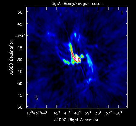
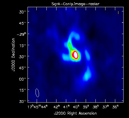
The clean images, shown in Fig. 2a-c, give a first impression of the data. Note that when combining the images, we will improve on the uv-coverage and will therefore not only combine high resolution with high surface brightness sensitivity on large scales, but also expect a higher image fidelity, i.e. fewer artifacts due to better deconvolution.
The basic parameters of the individual images can be checked through imhead for the spatial resolution and determining the rms when checking the statistics of empty areas within the viewer. The central point source, Sgr A*, is variable and we see this reflected in the flux density values from the images taken in the three different configurations, which were separated in observing time by several months:
A-configuration: synthesized beam  1.44" x 0.40"; rms ~0.8mJy; peak flux density of Sgr A* 0.712 Jy/beam
B-configuration: synthesized beam  4.33" x 1.34"; rms ~0.7mJy; peak flux density of Sgr A* 0.691 Jy/beam
C-configuration: synthesized beam 11.02" x 4.20"; rms ~0.6mJy; peak flux density of Sgr A* 1.35 Jy/beam
Removal of the variable Sgr A* point source
This step is only necessary for our case which includes a variable source. In most cases, one can skip this step.
We have seen in the initial images that Sgr A* is a variable source. This introduces some problems for data combination as the visibilities of the different sessions will reflect these variations. Cleaning will be difficult in such a situation as flux levels at different uv points (times and baselines) are not consistent in their portion for the central point source. Therefore, we will remove the unresolved Sgr A* in each dataset. For those who are interested in having Sgr A* back in the image, we will later show how to re-introduce a nominal point source with a flux of 1Jy. It is perfectly fine, however, to image without the artificial source.
To start, we create a component list for each dataset that includes only a point source at the position of Sgr A*. To do so, we first need to find out the position of the central point source. This is performed by fitting a point source (2d-Gaussian function) to the A-configuration data, which has the largest angular resolution. We use imfit:
# In CASA
imfit(imagename='SgrA-Aonly.image',box='630,620,650,660')
The output of imfit into the logger is as follows:
Fit on SgrA-Aonly.image component 0
Position ---
       --- ra:    17:45:40.038547 +/- 0.000059 s (0.000777 arcsec along great circle)
       --- dec: -029.00.28.051226 +/- 0.004597 arcsec
       --- ra:  639.9677 +/- 0.0078 pixels
       --- dec: 640.1777 +/- 0.0460 pixels
We will be using RA (J2000) =17h45m40.038547s and DEC (J2000) = -29d00'28.051226" for the central position of Sgr A*. We will use these coordinates for all three configurations, although it might be advisable to fit each dataset separately in case the peak may slightly shift. In this case, a single position works for all of our three data sets.
The component list will be inserted as a MODEL column into the respective MS via ft. Task uvsub will then be used to subtract the point source model from the CORRECTED data column. Since there's no CORRECTED column to start with, uvsub will initially copy the DATA column to the CORRECTED column, then subtract. Note that running uvsub twice will oversubtract; we recommend to create backup copies of the previous datasets before subtracting Sgr A*:
# In a Terminal
cp -r VLA-SgrA-Sband-Aconfig.ms VLA-SgrA-Sband-Aconfig-sub.ms
cp -r VLA-SgrA-Sband-Bconfig.ms VLA-SgrA-Sband-Bconfig-sub.ms
cp -r VLA-SgrA-Sband-Cconfig.ms VLA-SgrA-Sband-Cconfig-sub.ms
Let's start with the A-configuration data and create a component list of a point source with a flux of 0.712 Jy at a position of RA (J2000) =17h45m40.038547s and DEC (J2000) = -29d00'28.051226" (more examples of component lists are provided in the CASA guide Create a Component List for Selfcal):
# In CASA
cl.addcomponent(flux=0.712, fluxunit='Jy',shape='point', dir='J2000 17:45:40.038547 -29.00.28.051226')
cl.rename('component-SgrA-A.cl')
cl.close()
(We have used the CASA coordinate convention with colons for h:m:s and dots for d.m.s.)
The component list is now stored in the file 'component-SgrA-A.cl' and we will use it to populate the MODEL column via ft:
# In CASA
ft(vis='VLA-SgrA-Sband-Aconfig-sub.ms', complist='component-SgrA-A.cl', usescratch=True)
At this step the MODEL column is created.
Finally we will subtract the MODEL from the DATA/CORRECTED_DATA with uvsub. This task will also create CORRECTED as it does not exist yet:
# In CASA
uvsub(vis='VLA-SgrA-Sband-Aconfig-sub.ms')
Note that to revert back to the original state, you can use task clearcal to reset the MODEL column and to set CORRECTED to be identical with DATA (thus undoing the source subtraction).
Let's repeat the steps for B-configuration, now using a flux of 0.691 Jy. Although a separate fit would be even better, the subtraction also works well when using the A-configuration position:
# In CASA
cl.addcomponent(flux=0.691, fluxunit='Jy',shape='point', dir='J2000 17:45:40.038547 -29.00.28.051226')
cl.rename('component-SgrA-B.cl')
cl.close()
#
ft(vis='VLA-SgrA-Sband-Bconfig-sub.ms', complist='component-SgrA-B.cl', usescratch=True)
#
uvsub(vis='VLA-SgrA-Sband-Bconfig-sub.ms')
And for C-configuration we subtract a point source of 1.35 Jy (note that the central flux includes some extended emission, but is still dominated by Sgr A*):
# In CASA
cl.addcomponent(flux=1.35, fluxunit='Jy',shape='point', dir='J2000 17:45:40.038547 -29.00.28.051226')
cl.rename('component-SgrA-C.cl')
cl.close()
#
ft(vis='VLA-SgrA-Sband-Cconfig-sub.ms', complist='component-SgrA-C.cl', usescratch=True)
#
uvsub(vis='VLA-SgrA-Sband-Cconfig-sub.ms')
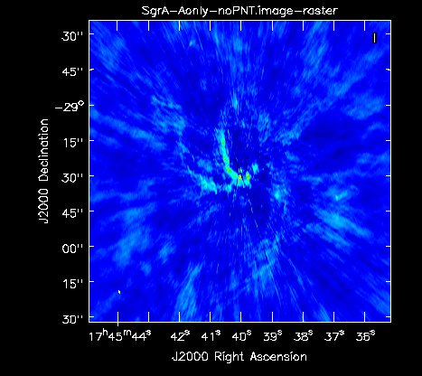
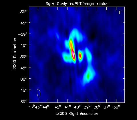
Let's image the three data sets with Sgr A* removed. We will run tclean, but since the point source is removed, we only do 500 iterations for A and B configurations, and 200 iterations for the C configuration data to avoid cleaning into the noise:
# In CASA
# A-config:
tclean(vis='VLA-SgrA-Sband-Aconfig-sub.ms', imagename='SgrA-Aonly-noPNT',field='J1745-2900',
      specmode='mfs',cell='0.1arcsec',imsize=[1280,1280],niter=500,weighting='briggs',robust=0)
# In CASA
# B-config:
tclean(vis='VLA-SgrA-Sband-Bconfig-sub.ms', imagename='SgrA-Bonly-noPNT',field='J1745-2900',
      specmode='mfs',cell='0.1arcsec',imsize=[1280,1280],niter=500,weighting='briggs',robust=0)
# In CASA
# C-config:
tclean(vis='VLA-SgrA-Sband-Cconfig-sub.ms', imagename='SgrA-Conly-noPNT',field='J1745-2900',
      specmode='mfs',cell='0.1arcsec',imsize=[1280,1280],niter=200,weighting='briggs',robust=0)
As expected, the images without the point sources as shown in Fig. 3a-c look similar to those in Fig. 2a-c. but with the central point source removed. Since we cleaned a given number of iterations, some differences are visible, particularly for C-configuration. This is expected.
Check and Adjust the Visibility Weights
VLA weights are currently based only on channel width and correlator integration time. In the future, the VLA may use the switched power measurements to derive absolute calibrated weights. At the moment, however, the VLA weights need to be taken as being relative to each other. The relative sensitivity within an observation is measured by the gain, so weights of single, continuous observations are self-consistent. It is important to adjust the weights between separate observations as they will be on different scales.
Let's have a look at the weights of the different datasets. We will plot the weights as a function of uv-distance for a single spectral window (spw='3'), average over all channels in one spectral window, and will colorize by antenna:
# In CASA
# A-config:
plotms(vis='VLA-SgrA-Sband-Aconfig-sub.ms',spw='3',averagedata=True,
       avgchannel='64',xaxis='uvwave',yaxis='wt',coloraxis='antenna1')
# In CASA
# B-config
plotms(vis='VLA-SgrA-Sband-Bconfig-sub.ms',spw='3',averagedata=True,
       avgchannel='64',xaxis='uvwave',yaxis='wt',coloraxis='antenna1')
# In CASA
# C-config:
plotms(vis='VLA-SgrA-Sband-Cconfig-sub.ms',spw='3',averagedata=True,
       avgchannel='64',xaxis='uvwave',yaxis='wt',coloraxis='antenna1')
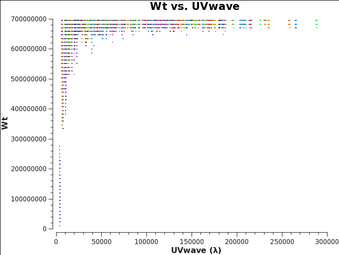
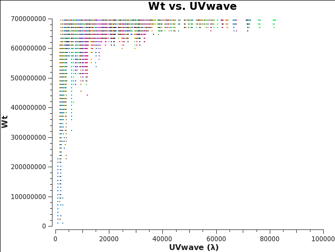
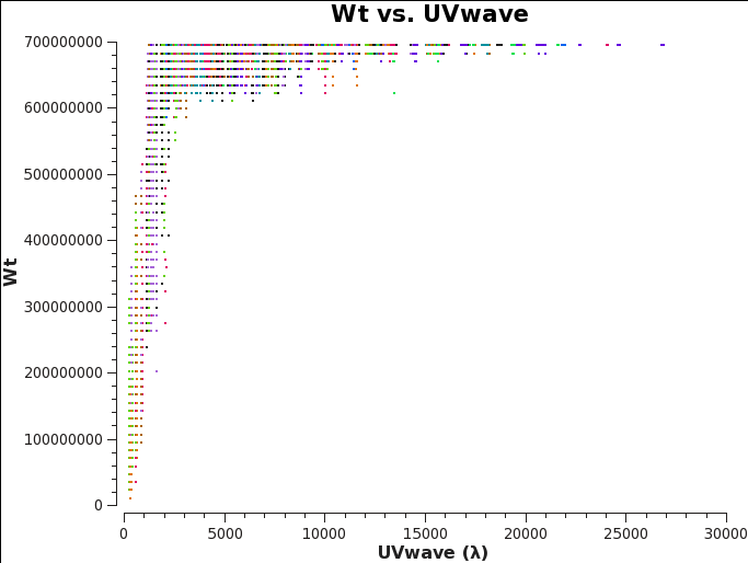
Fig. 4a-c shows that there are some differences. Data from configurations A and B have weights that are reasonably comparable. C-configuration data, however, seems to have consistently lower values.
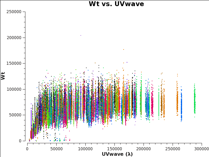 A-config original weights. |
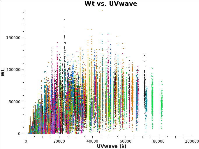 B-config original weights. |
 C-config original weights. |
The next step is to bring the weights on the same relative scale. There are currently a number of options to do so.
1) Reset the weights with initweights to reflect the channel width and correlator integration time ([math]\displaystyle{ WEIGHT=2 \Delta \nu \Delta t }[/math], see the document on Data Weights in CASAdocs).
2) Calculate the weights based on the rms of the visibilities themselves, using the statwt task.
3) Calculate the weights based on the rms of the cross-polarization products (currently not supported in statwt).
We recommend to reset the weights when there are strong sources present in the data as they will change the rms of the visibilities and the rms will not be representative of the noise anymore. Without strong sources, statwt should deliver better results. The third option may work both cases, but requires full polarization observations and calibrations. For this guide we will perform the first two options and compare the results. Our data has no cross-polarization products, so the third option is not applicable.
Option 1: Resetting the weights
As we will overwrite the WEIGHT column, we first create copies of our MSs in case we will have to revert to the original data:
# In a Terminal
cp -r VLA-SgrA-Sband-Aconfig-sub.ms VLA-SgrA-Sband-Aconfig-sub-initwt.ms
cp -r VLA-SgrA-Sband-Bconfig-sub.ms VLA-SgrA-Sband-Bconfig-sub-initwt.ms
cp -r VLA-SgrA-Sband-Cconfig-sub.ms VLA-SgrA-Sband-Cconfig-sub-initwt.ms
Now we will reset the weights with initweights. Parameter wtmode='nyq' is the default and resets the weights based on the channel width and correlator integration time (see above).
# In CASA
# A-config:
initweights(vis='VLA-SgrA-Sband-Aconfig-sub-initwt.ms',wtmode='nyq')
# In CASA
# B-config:
initweights(vis='VLA-SgrA-Sband-Bconfig-sub-initwt.ms',wtmode='nyq')
# In CASA
# C-config:
initweights(vis='VLA-SgrA-Sband-Cconfig-sub-initwt.ms',wtmode='nyq')
Let's have a look at the weight values again to see if initweights has reset the weights properly:
First, let's plot every visibility (Figure 5a):
# In CASA
# A-config:
plotms(vis='VLA-SgrA-Sband-Aconfig-sub-initwt.ms',spw='3',xaxis='uvwave',yaxis='wt',coloraxis='antenna1')
And now, let's average across channels
# In CASA
# A-config:
plotms(vis='VLA-SgrA-Sband-Aconfig-sub-initwt.ms',spw='3',averagedata=True,
       avgchannel='64',xaxis='uvwave',yaxis='wt',coloraxis='antenna1')
# In CASA
# B-config
plotms(vis='VLA-SgrA-Sband-Bconfig-sub-initwt.ms',spw='3',averagedata=True,
       avgchannel='64',xaxis='uvwave',yaxis='wt',coloraxis='antenna1')
# In CASA
# C-config:
plotms(vis='VLA-SgrA-Sband-Cconfig-sub-initwt.ms',spw='3',averagedata=True,
       avgchannel='64',xaxis='uvwave',yaxis='wt',coloraxis='antenna1')
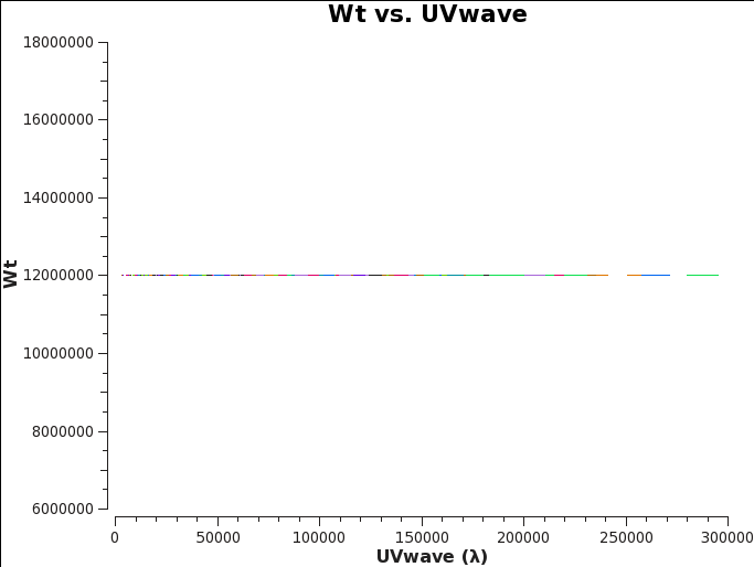 Weights after they were reset. |
The weights are plotted in Fig. 5a for one configuration and per channel. They are identical for all data sets, as the data were taken in the same way for all configurations with 3s correlator integration time and 2MHz channel width. According to the equation above, this amounts to a weight of 1.2e7 for all visibilities. Figures 5b,c, and d show the weights for channel-averaged data. Note that the correct weights are the sums across all 64 channels, which adds up to ~7e8. Flagged channels are reducing the weights.
Option 2: Calculating the weights based on the rms
The second option to bring all weights on the same scale involves the execution of the CASA task statwt. This task recalculates the visibility weights based on their rms. Task statwt is part of the VLA pipeline, which was used to calibrate the original data. This explains the similarity of the A and B configuration weights in Fig. 4a and b. We will nevertheless run statwt once more on all files in order to ensure proper compatibility of the data (older versions of CASA may have been used for the pipeline, and CASA underwent major changes in its definition of data weights).
Task statwt will be executed on each MS. The default setting calculates the weight based on the rms of each scan and spectral window. This setting works quite well for continuum observations. We would like to note though that for spectral line data the fitspw parameter should be set to exclude the line from the calculations. Otherwise, strong lines will be down-weighted.
As statwt will overwrite the WEIGHT column, we once more create copies of our MSs in case we will have to revert to the original data:
# In a Terminal
cp -r VLA-SgrA-Sband-Aconfig-sub.ms VLA-SgrA-Sband-Aconfig-sub-statwt.ms
cp -r VLA-SgrA-Sband-Bconfig-sub.ms VLA-SgrA-Sband-Bconfig-sub-statwt.ms
cp -r VLA-SgrA-Sband-Cconfig-sub.ms VLA-SgrA-Sband-Cconfig-sub-statwt.ms
Now, we execute statwt on the new datasets:
# In CASA
# A-config:
statwt(vis='VLA-SgrA-Sband-Aconfig-sub-statwt.ms')
# In CASA
# B-config
statwt(vis='VLA-SgrA-Sband-Bconfig-sub-statwt.ms')
# In CASA
# C-config:
statwt(vis='VLA-SgrA-Sband-Cconfig-sub-statwt.ms')
Let's have a look at the weight values again to see if statwt has adjusted the weights properly:
# In CASA
# A-config:
plotms(vis='VLA-SgrA-Sband-Aconfig-sub-statwt.ms',spw='3',averagedata=True,
       avgchannel='64',xaxis='uvwave',yaxis='wt',coloraxis='antenna1')
# In CASA
# B-config
plotms(vis='VLA-SgrA-Sband-Bconfig-sub-statwt.ms',spw='3',averagedata=True,
       avgchannel='64',xaxis='uvwave',yaxis='wt',coloraxis='antenna1')
# In CASA
# C-config:
plotms(vis='VLA-SgrA-Sband-Cconfig-sub-statwt.ms',spw='3',averagedata=True,
       avgchannel='64',xaxis='uvwave',yaxis='wt',coloraxis='antenna1')
In Fig. 6a-c we plot the new, recalculated weights for the three configurations. The absolute scaling has indeed changed, likely due to a different weight definition that was used in earlier versions of CASA when the data were calibrated. The relative weights between A and B configurations still appear to be similar to the original, relative numbers. The C-configuration weights, however, appear to be slightly lower relative to A and B, likely due to more flux in the MS.
 A-config recalculated weights. |
 B-config recalculated weights. |
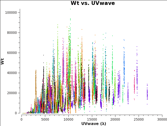 C-config recalculated weights. |
Combining and Imaging All Data
We will now create a combined image of all three re-weighted datasets.
First, let's check the new uv-coverage. We need to concatenate the data with concat (alternatively, one can use virtualconcat, a task that can also concatenate multi-MSs). We concatenate both the datasets with initialized weights as well as those with re-computed weights:
# In CASA
concat(vis=['VLA-SgrA-Sband-Aconfig-sub-initwt.ms','VLA-SgrA-Sband-Bconfig-sub-initwt.ms','VLA-SgrA-Sband-Cconfig-sub-initwt.ms'],concatvis='VLA-SgrA-Sband-initwt-combined.ms')
#
concat(vis=['VLA-SgrA-Sband-Aconfig-sub-statwt.ms','VLA-SgrA-Sband-Bconfig-sub-statwt.ms','VLA-SgrA-Sband-Cconfig-sub-statwt.ms'],concatvis='VLA-SgrA-Sband-statwt-combined.ms')
Now let's plot the uv-coverage of one of the combined MSs, e.g.:
# In CASA
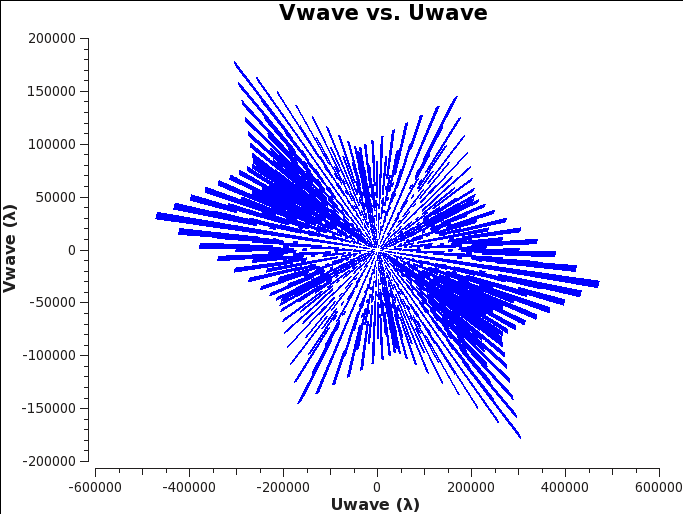
plotms(vis='VLA-SgrA-Sband-initwt-combined.ms',xaxis='Uwave',yaxis='Vwave',plotrange=[-600000,600000,-200000,200000])
Fig. 7 shows the combined uv-coverage, which extends to A-configuration baselines but with a much higher density at the intermediate and shorter baselines contributed from B and C configurations.
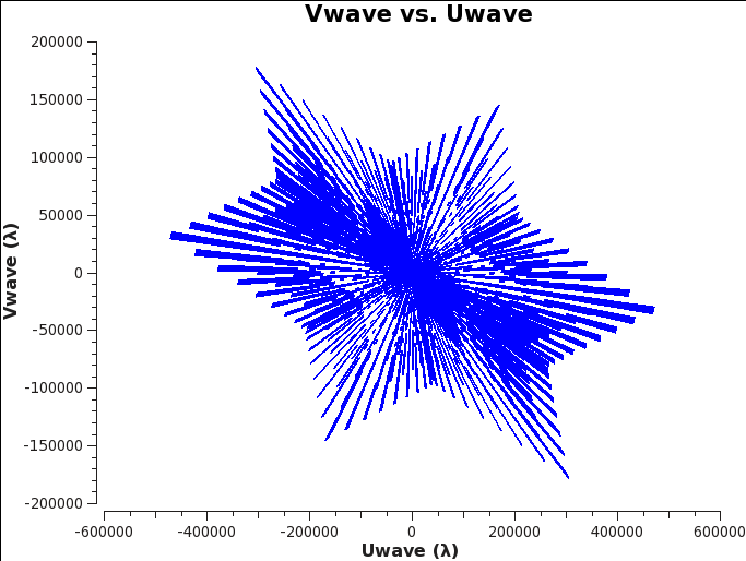 Combined uv-coverage. |
Although concat merges all three MSs into a single one, it is actually not a required step before imaging. Task tclean will take care of the combination when all datasets are specified as a list. By default, tclean will image the data in the CORRECTED columns, i.e. it will use the portion of the MS which exhibits the data with the subtracted Sgr A* point source (if CORRECTED is not present, it will image the visibilities stored in the DATA column). Tclean will also perform the spectral regridding of all datasets on the fly, in particular in mode="velocity" or mode="frequency". There's no need to run cvel/cvel2 (or mstransform) to Doppler correct the MSs beforehand.
We will now create a combined image in tclean. The threshold parameter was derived by a previous run of tclean on the combined MS for which we determined the rough rms noise. For our threshold, we will use the rms noise multiplied by a factor of ~2.5.
Let's start with the data with weights that were reset:
# In CASA
tclean(vis=['VLA-SgrA-Sband-initwt-combined.ms'],
      imagename='GC-initwt-all',field='J1745-2900',specmode='mfs',cell='0.1arcsec',imsize=[1280,1280],niter=3000,
      threshold='5mJy',weighting='briggs',robust=0)
And now we image the data with recalculated weights:
# In CASA
tclean(vis=['VLA-SgrA-Sband-statwt-combined.ms'],
      imagename='GC-statwt-all',field='J1745-2900',specmode='mfs',cell='0.1arcsec',imsize=[1280,1280],niter=3000,
      threshold='5mJy',weighting='briggs',robust=0)
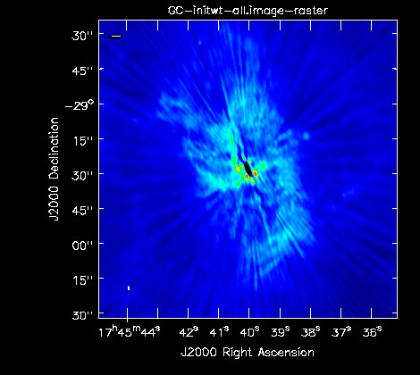
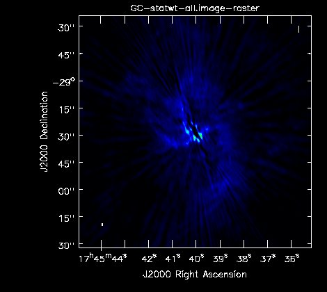
The resulting images look somewhat different when plotted on the same scales (Fig. 8a-b). To start, the beams are 1.74"x0.61" for the one with initialized data weights and 1.58"x0.50" for the one with statwt computed weights. Those values are similar to the resolution of A-configuration only, but we do note that the one with the larger beam also shows the extended emission more prominently. The rms is ~2mJy and thus better than A-only for the initialized weights image (about a factor of 2 less for the statwt image) and there are clearly many more extended spatial scales in both images.
These images can still be improved upon. For simplicity, we did not use any interactive cleaning in the above, but we highly recommend it for producing the final images. Improvements can also be obtained by adjusting the image weights via the Briggs robust parameter, adding a taper, or weighting the different datasets against each other using visweightscale in concat. Wide-band imaging and multi-scale imaging will also lead to better results. We refer to the VLA CASA Imaging Guide for more details and examples.
Inserting an artificial Point Source for Sgr A*
Finally, we will add in a point source with a canonical flux density of 1 Jy to bring back Sgr A*. We again create a component list and use ft to attach the source model. Using uvsub with reverse=True will add instead of subtract the MODEL to DATA/CORRECTED. This step can be skipped when Sgr A* is not required. When the data are going to be self-calibrated, we actually recommend to not introduce an artificial source during the calibration steps as it has no phase errors imprinted. For this example, we now re-introduce Sgr A*. Once more, we start by copying the combined datasets:
# In a Terminal
cp -r VLA-SgrA-Sband-initwt-combined.ms VLA-SgrA-Sband-initwt-combined-addPNT.ms
cp -r VLA-SgrA-Sband-statwt-combined.ms VLA-SgrA-Sband-statwt-combined-addPNT.ms
Now we create a component list with a 1 Jy point source at the previously derived position of Sgr A*.
# In CASA
cl.addcomponent(flux=1, fluxunit='Jy',shape='point', dir='J2000 17:45:40.038547 -29.00.28.051226')
cl.rename('component-SgrA.cl')
cl.close()
Finally, we insert it in the model column with ft and add it to the data with uvsub to both MSs, the one with initialized weights and the one with recomputed weights:
# In CASA
ft(vis='VLA-SgrA-Sband-initwt-combined-addPNT.ms', complist='component-SgrA.cl', usescratch=True)
#
uvsub(vis='VLA-SgrA-Sband-initwt-combined-addPNT.ms',reverse=True)
#
ft(vis='VLA-SgrA-Sband-statwt-combined-addPNT.ms', complist='component-SgrA.cl', usescratch=True)
#
uvsub(vis='VLA-SgrA-Sband-statwt-combined-addPNT.ms',reverse=True)
Now it is time to image both combined MSs once more:
# In CASA
tclean(vis=['VLA-SgrA-Sband-initwt-combined-addPNT.ms'],
      imagename='GC-initwt-all-addPNT',field='J1745-2900',specmode='mfs',cell='0.1arcsec',imsize=[1280,1280],niter=5000,
      threshold='5mJy',weighting='briggs',robust=0)
# In CASA
tclean(vis=['VLA-SgrA-Sband-statwt-combined-addPNT.ms'],
      imagename='GC-statwt-all-addPNT',field='J1745-2900',specmode='mfs',cell='0.1arcsec',imsize=[1280,1280],niter=5000,
      threshold='5mJy',weighting='briggs',robust=0)
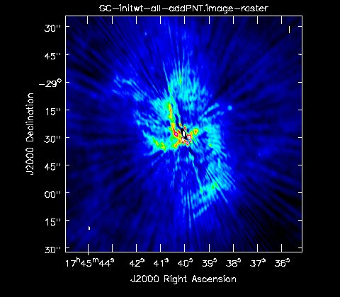
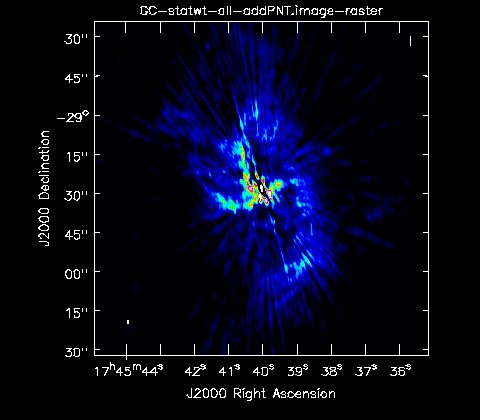
In Fig. 9a-b we show the resulting images on the same scales as in Fig. 8a-b. As expected the main difference is the added point source but some differences due to the tclean algorithm are also visible. Again, one can improve the images as described above.
Tips for Selfcal
If the source has a bright nucleus or, more generally, a bright unresolved emission, start with the A array data, selfcal, then add B array, selfcal again, and so on. This procedure starts with a high model flux that is increased further. If the source is mostly diffuse, then there is not much signal in the A array data, so start with the D array, selfcal, then add C array, selfcal, and so on. Each selfcal step should be phase only first with maybe two or more iterations. At the end of each selfcal step, a phase+amplitude selfcal can be attempted, before merging in the next array configuration data. After each merge the selfcal steps can be repeated.
In our case the steps would be done in the images which have Sgr A* removed; otherwise the variability of Sgr A* prevents such procedures. Also, when we replaced Sgr A* by an artificial 1 Jy source, that source will not have phase fluctuations imprinted and cannot be used for selfcal. It can be reintroduced as described above after all selfcal steps are completed.
Last checked on CASA Version 5.5.0.

