PlotWVRSolutions: Difference between revisions
No edit summary |
|||
| (2 intermediate revisions by 2 users not shown) | |||
| Line 3: | Line 3: | ||
This page documents the '''plotWVRSolutions''' function of Python module [[Analysis Utilities|analysisUtils]]. | This page documents the '''plotWVRSolutions''' function of Python module [[Analysis Utilities|analysisUtils]]. | ||
Although plotcal can be used to plot the ALMA WVR solutions on an antenna-basis, it is often not very insightful because it includes the common-mode changes in atmospheric delay above the array which | Although plotcal can be used to plot the ALMA WVR solutions on an antenna-basis, it is often not very insightful because it includes the common-mode changes in atmospheric delay above the array which can be large enough that it becomes hard to see temporal differences between antennas. The function plotWVRSolutions takes pairwise difference between antennas and produces plots of the effective phase correction on a baseline basis. The plots can be sorted by antenna number pair (default) or by baseline length. Fields are plotted in different colors. All spws are displayed sequentially, so be sure to limit them to (one of) the science spws, because they should only differ by the frequency ratio. | ||
==Usage== | ==Usage== | ||
| Line 13: | Line 13: | ||
plotWVRSolutions(caltable='', spw=[], field=[], subplot=22, sort='number', antenna='', | plotWVRSolutions(caltable='', spw=[], field=[], subplot=22, sort='number', antenna='', | ||
xrange=[0, 0], yrange=[0, 0], figfile='', help=False, | xrange=[0, 0], yrange=[0, 0], figfile='', help=False, | ||
xaxis='ut', interactive=True) | xaxis='ut', interactive=True, ms='') | ||
Options: | Options: | ||
antenna: can be ID or name; single value, or list: 0,'0','0,1','DV04,DV05'. | antenna: can be ID or name; single value, or list: 0,'0','0,1','DV04,DV05'. | ||
| Line 20: | Line 20: | ||
figfile: will append .0.png, .1.png, etc. for successive pages | figfile: will append .0.png, .1.png, etc. for successive pages | ||
interactive: True or False (True will require user input after showing each page) | interactive: True or False (True will require user input after showing each page) | ||
ms: specify the ms name rather than look for it in the caltable | |||
sort: by baseline 'number', or by baseline 'length' | sort: by baseline 'number', or by baseline 'length' | ||
subplot: valid values: 11,12,21,22,23,32,42 (any 3rd digit is ignored) | subplot: valid values: 11,12,21,22,23,32,42 (any 3rd digit is ignored) | ||
| Line 33: | Line 34: | ||
<source lang="python"> | <source lang="python"> | ||
# In CASA | # In CASA | ||
au.plotWVRSolutions('wvr_X3c1.cal',field='!3c279',spw='17') | au.plotWVRSolutions('wvr_X3c1.cal',field='!3c279',spw='17',figfile='X3c1.wvr') | ||
</source> | </source> | ||
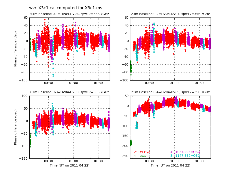
Here is the first page of plots generated by this command: | |||
[[File: X3c1.wvr.0.png]] | |||
Latest revision as of 13:51, 6 April 2017
Return to Analysis Utilities
This page documents the plotWVRSolutions function of Python module analysisUtils.
Although plotcal can be used to plot the ALMA WVR solutions on an antenna-basis, it is often not very insightful because it includes the common-mode changes in atmospheric delay above the array which can be large enough that it becomes hard to see temporal differences between antennas. The function plotWVRSolutions takes pairwise difference between antennas and produces plots of the effective phase correction on a baseline basis. The plots can be sorted by antenna number pair (default) or by baseline length. Fields are plotted in different colors. All spws are displayed sequentially, so be sure to limit them to (one of) the science spws, because they should only differ by the frequency ratio.
Usage
CASA <8>: help(au.plotWVRSolutions)
Help on function plotWVRSolutions in module analysisUtils:

plotWVRSolutions(caltable='', spw=[], field=[], subplot=22, sort='number', antenna='',
                 xrange=[0, 0], yrange=[0, 0], figfile='', help=False,
                 xaxis='ut', interactive=True, ms='')
  Options:
    antenna: can be ID or name; single value, or list: 0,'0','0,1','DV04,DV05'.
             Accepts the standard '!' modifier, but not '&'.
    field: must be field ID, or list of IDs, or comma-delimited string of IDs
    figfile: will append .0.png, .1.png, etc. for successive pages
    interactive: True or False (True will require user input after showing each page)
    ms: specify the ms name rather than look for it in the caltable
    sort: by baseline 'number',  or by baseline 'length'
    subplot:   valid values: 11,12,21,22,23,32,42  (any 3rd digit is ignored)
    xaxis: 'seconds' or 'ut' (default)
    xrange: min/max time to show:  specify in seconds if xaxis='seconds'
            or floating point UT hours if 'ut'.  The latter will
            probably not work well if the data cross the 0/24 hour mark.
    yrange: min/max phase to show
Examples
# In CASA
au.plotWVRSolutions('wvr_X3c1.cal',field='!3c279',spw='17',figfile='X3c1.wvr')
Here is the first page of plots generated by this command:
