VLA Polarization pipe Tutorial
Notes on CASA
This CASA Guide is for Version 6.4.1 of CASA. If you are using a later version of CASA and this is the most recent available guide, then you should be able to use most, if not all, of this tutorial. This guide is meant to be completed using the monolithic CASA and not modular CASA as the GUI may not work correctly otherwise.
There are a number of possible ways to run CASA, described in more detail in Getting Started in CASA. In this tutorial we would like you to use either (or both) of the following methods so that you can familiarize yourself with the CASA software:
- Interactive: examining task inputs. In this mode, one types taskname to load the task, inp to examine the inputs, and go once those inputs have been set to your satisfaction. Allowed inputs are shown in blue and bad inputs are colored red. The input parameters themselves are changed one by one, e.g., selectdata=True. Screenshots of the inputs to various tasks used in the data reduction below are provided, to illustrate which parameters need to be set. More detailed help can be obtained on any task by typing help taskname. Once a task is run, the set of inputs is stored and can be retrieved via tget taskname; subsequent runs will overwrite the previous tget file.
- Pseudo-interactive: task function calls. In this mode, all of the desired inputs to a task are provided at once inn the CASA command line. This tutorial is made up of such calls, which were developed by looking at the inputs for each task and deciding what needed to be changed from default values. For task function calls, only parameters that you want to be different from their defaults need to be set.
This tutorial is largely self-paced. Any time you have a question, or something doesn't look right or you are unsure of, please do summon one of the tutors present in the room.
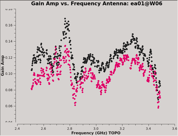
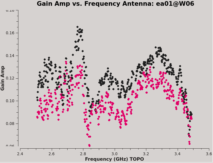
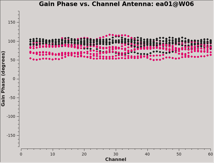
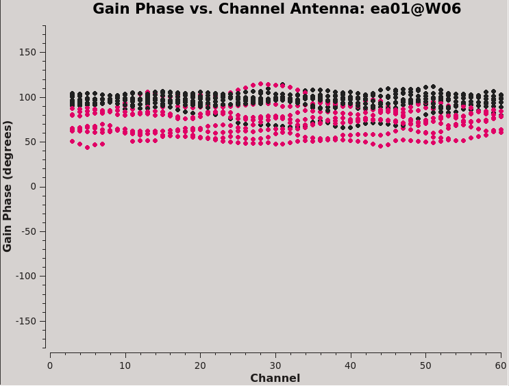
Data Set
This CASA guide describes the calibration and imaging of a single-pointing continuum data set taken with the Karl G. Jansky Very Large Array (VLA) of the binary black hole system 3C 75 in Abell 400 cluster of galaxies [1]. The observations were performed with a single 1 GHz baseband centered at 3.0 GHz, resulting in 8x128 MHz wide spectral windows with 64 channels each. The observation was set up to allow for full polarization calibration.
Prior to the synthesis imaging workshop you should have received instructions to download the data for this tutorial. If you have not already, you will need to untar and unzip the file using the command: 'tar -xzvf TDRW0001_calibrated_CASA6.4.1.ms.tgz' and then give it the same name as the guide uses: 'mv TDRW0001_calibrated_CASA6.4.1.ms TDRW0001_calibrated.ms'.
The first step of polarization calibration is to first obtain a decent Stokes I (RR and LL) calibration. This has already been done for you by running the raw data through the CASA 6.4.1 version of the VLA pipeline. One additional step was required which involved removing the parallactic angle correction that was applied by the standard pipeline. For those familiar with the VLA pipeline, we essentially repeated what pipeline tasks hifv_applycals, hifv_targetflag, and hifv_statwt did, but disabled the application of parallactic angle corrections.
The Observation
Before starting the calibration process, we want to get some basic information about the data set. To examine the observing conditions during the observing run, and to find out any known problems with the data, we can take a look at the observer log, but in order to get to our observation we'll need the date it was observed on. The CASA task to use to get that information, and other very useful information on the setup of the observation is: listobs.
Once you've gotten the date of observation for this data set find its observer log and note the two antennas that had issues during the observation.
Before beginning our polarization calibration, we should inspect the pipeline calibration weblog for any obvious issues. You can download the weblog from ['https://casa.nrao.edu/Data/VLA/Polarization/SIW19pipeline-20230103T175723.tgz '] or view it through a browser here. For those not familiar with viewing these weblogs, they are basically a little report that is meant to help judge how well the VLA pipeline did with its calibration. Feel free to explore it as you wish, but you'll likely find two of the more useful stages to look at are hifv_finalcals (plots of the final solution tables) and hifv_plotsummary (various plots of the calibrated data). For more details on the pipeline output you can have a look at the VLA CASA Pipeline Guide.
You will likely note that there are four sources observed. Here the sources are introduced briefly, with more detail contained in the sections below in which they are used:
- 0137+331=3C48, which will serve as a calibrator for the visibility amplitudes, i.e., it is assumed to have precisely known flux density, the spectral bandpass, and the polarization position angle;
- J0259+0747, which will serve as a calibrator for the visibility phases and can be used to determine the instrumental polarization;
- J2355+4950, which can serve as a secondary instrumental polarization calibrator or to check residual instrumental polarization, and;
- 3C75, which is the science target.
Both to get a sense of the array, as well as identify the location of the reference antenna that we told the pipeline to choose for parallel hand calibration, have a look at the antenna setup page of the weblog. For calibration purposes, you would generally select an antenna that is close to the center of the array (and that is not listed in the operator's log as having had problems!).
Can you tell which antenna we chose for our reference antenna?
The reference antenna by definition has its delays and phases set to zero. So by looking at those solution tables in the hifv_finalcals stage we can see that ea10 was our reference antenna.
Examining and Editing the Data
It is always a good idea to examine the data before jumping straight into calibration. Even though the pipeline did a good job of calibrating and flagging the data, it isn't perfect. From the pipeline weblog, looking at the final amplitude gain calibration vs time plots in hifv_finalcals, we can see that during the second half of the observation antennas ea03, ea12, and ea16 shows some gain instability; otherwise there are no issues identified at this point.
We will start by making a simple overview plot.
# In CASA
plotms(vis='TDRW0001_calibrated.ms', selectdata=True, correlation='RR', averagedata=True, avgchannel='64', coloraxis='field', plotfile='colorbyfield.jpeg')
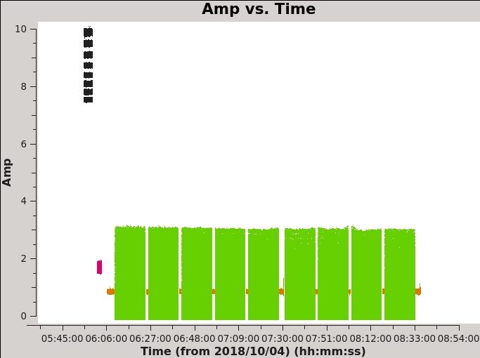
- selectdata=True : One can choose to plot only selected subsets of the data.
- correlation='RR' : Plot only the right-handed (left-handed omited only for speed) polarization products. The cross-terms ('RL' and 'LR') will be close to zero for non-polarized sources.
- averagedata=True: One can choose to average data points before plotting them.
- avgchannel='64' : With this plot, we are mainly interested in the fields vs time. Averaging over all 64 channels in the spectral window makes the plotting faster.
- coloraxis='field' : Color-code the plotting symbols by field name/number.
The default x- and y-axis parameters are 'time' and 'amp', so the above call to plotms produces an amplitude vs time plot of the data for a selected subset of the data (if desired) and with data averaging (if desired). Many other values have been left to defaults, but it is possible to select them from within the plotms GUI.
Based on what you've learned from the listobs task you should be able to tell which sources are which in the plot.
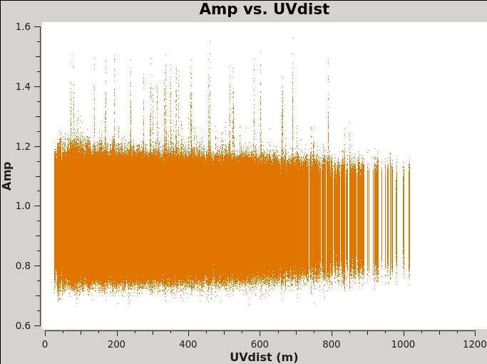
Another example of using plotms for a quick look at your data, select the Data tab and specify field 2 (the complex gain calibrator J0259+0747) to display data associated with the target, then select the Axes tab and change the X-axis to be UVdist (baseline length in meters). Remove the channel averaging (Data tab), and plot the data using the Plot button at the bottom of the plotms GUI. The important observation is that the amplitude distribution is relatively constant as a function of UV distance or baseline length (i.e., [math]\displaystyle{ \sqrt{u^2+v^2} }[/math]; see Figure 2A). A relatively constant visibility amplitude as a function of baseline length means that the source is very nearly a point source (the Fourier transform of a point source, i.e. a delta function, is a constant function). You can see occasional spikes in the calibrated amplitudes. This is most likely caused by radio frequency interference that correlates on certain baselines. We will get to those further in the guide.
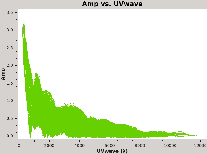
By contrast, if you make a similar plot for field 3 (our target 3C 75), the result is a visibility function that falls rapidly with increasing baseline length. Figure 2B shows this example, including time averaging of '1e6' seconds (any large number that encompasses more than a full scan will do, we want to fully average each scan). Such a visibility function indicates a highly resolved source. To plot baseline length in wavelengths rather than meters, select UVwave as the X-axis parameter.
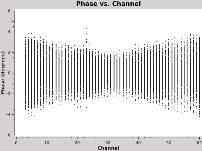
A final example is shown in Figure 2C. In this example, we have elected to show phase as a function of (frequency) channel for a single baseline (antenna='ea01&ea21' ) on the bandpass calibrator, field 0, and non-averaged data. If you choose to iterate by baseline (e.g., antenna='ea01' and iteraxis='baseline' ), you can see similar phase-frequency variations on all baselines. They center around zero phase, because we are looking at the calibrated visibilities; however, you are seeing a butterfly shaped pattern with phase noise higher toward the channel edges. This pattern is due to a small mismatch in the delay measurement timing (also known as 'delay clunking') which is an internally generated effect and is typically averaged out over time.
On Figure 1 you'll notice that the sources colored in black and green show much more spread in amplitude as compared to the others. Do you know the cause of this?
The black source is our flux density scale and bandpass calibrator, 3C48, and the green source is our target, 3C75. As we saw in Figure 2B, the spread in amplitude of 3C75 is primarily due to the presence of extended structure, that is to say, every baseline sees a slightly different amplitude. However if you make a similar plot of 3C48 you'll notice it is a point source. The spread on it is due to its spectral index (coloring by spectral window should make this stand out).
You can find similar plots in the CASA pipeline weblog under the task hifv_plotsummary. At this stage the pipeline has taken care of most of the calibration. There might be some remaining issues though that were not caught by the pipeline. In the following we note a couple issues that you might have found while inspecting data in this section. We will take care of those through additional flagging.
Issues that you might find:
 - ea12, scan 17: amplitude spike at the end of the scan (can be spotted already in Figure 1)
 - Residual RFI (see Figure 2A)
In the case of the amplitude spike, we can flag the affected time period by invoking the casa task flagdata. It is a good idea to save the original flags before performing any flagging by setting flagbackup=True.
# In CASA
flagdata(vis='TDRW0001_calibrated.ms', flagbackup=True, mode='manual', antenna='ea12',scan='17',timerange='07:25:57~07:26:18')
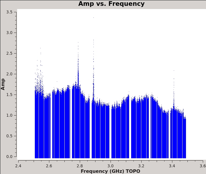
You can check the effect of this flagging by replotting Figure 2A. The spikes we saw before on some baselines should have disappeared. If you plot frequency against amplitude without averaging, however, you will still see some channels with interference that we will need to flag, especially on the instrumental polarization calibrators. Polarization calibration is very sensitive to interference, especially in the cross-hand correlations RL,LR. The pipeline does a good job at this, but there are still some RFI left; we will perform some additional flagging steps in the next section.
Additional Flagging
First we try to get a good sense of additional flagging that might be needed by plotting frequency against amplitude for the RR,LL and RL,LR polarizations of our calibrators (fields 0 through 2). You will notice some left over RFI on the bandpass calibrator in RR, LL. However, we also need to pay particular attention to RL, LR (see Figure 4A). Here we consider calibrators only; we will perform additional flagging on the target field at a later stage.
# In CASA
# for parallel hands
plotms(vis='TDRW0001_calibrated.ms',xaxis='frequency',yaxis='amplitude',field='0~2',correlation='RR,LL')
# for cross-hands
plotms(vis='TDRW0001_calibrated.ms',xaxis='frequency',yaxis='amplitude',field='0~2',correlation='RL,LR')
Since we are dealing with point sources, we do not have to worry about overflagging of shorter baselines, so we can run flagdata with mode='rflag' over the calibrator fields and cross-hand correlations to remove any residual RFI. For completeness, we also use mode='tfcrop' to reduce the amount of residual RFI in the parallel hands.
# In CASA

# for the parallel hands
flagdata(vis='TDRW0001_calibrated.ms',
	 mode='tfcrop',
	 field='0~2',
	 correlation='',
	 freqfit='line',
	 extendflags=False,
	 flagbackup=False)

# for the cross-hands
flagdata(vis='TDRW0001_calibrated.ms',
	 mode='rflag',
	 datacolumn='data',
	 field='0~2',
	 correlation='RL,LR',
	 extendflags=True,
	 flagbackup=False)
As you can see in Figure 4B, this additional flagging step took care of most of the obvious residual RFI. We are now ready to move on to calibrate the visibilities for linear polarization.
Polarization Calibration
Polarization calibration is done in three steps:

* First, we determine the instrumental delay between the two polarization outputs;

* Second, we solve for the instrumental polarization (the frequency-dependent leakage terms, 'D-terms'), using either an unpolarized source or a source which has sufficiently good parallactic angle coverage;

* Third, we solve for the polarization position angle using a source with a known polarization position angle (we use 3C48 here).
Before solving for the calibration solutions, we first use setjy to set the polarization model for our polarized position-angle calibrator. The pipeline only set the total intensity (Stokes I) of the flux density calibrator source 3C48, which did not include any polarization information. This source is known to have a fairly stable linear fractional polarization (measured to be 2% in S-band around the time of the observations), a polarization position angle of -100 degrees at 3 GHz, and a rotation measure of -68 rad/m^2. Note that 3C48 had an outburst in 2017 and is expected to show a significant degree of variability at higher frequencies in the first instance, progressively affecting lower frequencies as time passes since the event.
The setjy task will calculate the values of Stokes Q and U (in the reference channel) for user inputs of the reference frequency, Stokes I, polarization fraction, polarization angle, and rotation measure. It is possible to capture a frequency variation in Q, U, and alpha terms by providing coefficients of polynomial expansion for polarization fraction, polarization angle, and spectral index as a function of frequency. In general, it is left to the user to derive these coefficients, which can be accomplished by fitting a polynomial to observed values of the polarization fraction (here also called polarization index), polarization angle, and flux density (for the case of spectral index). These coefficients are then passed to the setjy task as lists along with the reference frequency and the Stokes I flux density.
As an example on how to derive the polarization parameters for the setjy call, you can perform the following next steps or jump right to the setjy call below.
Deriving the Polarization Properties of the Polarization Angle Calibrator
First, we tabulate the frequency dependent Stokes I flux density, polarization fraction, and polarization angle in a textfile, which we will call 3C48.dat. The data is taken from [2] and the corresponding Stokes I value is calculated from the Perley & Butler (2017) scale.
# Frequency  I       P.F.       P.A.
# (GHz)      (Jy)               (rad)
1.022        20.68   0.00293     0.07445
1.465        15.62   0.00457    -0.60282
1.865        12.88   0.00897     0.39760
2.565        9.82    0.01548    -1.97046
3.565        7.31    0.02911    -1.46542
4.885        5.48    0.04286    -1.24875
6.680        4.12    0.05356    -1.15533
8.435        3.34    0.05430    -1.10638
11.320       2.56    0.05727    -1.08602
14.065       2.14    0.06097    -1.09597
16.564       1.86    0.06296    -1.11891
19.064       1.67    0.06492    -1.18266
25.564       1.33    0.07153    -1.25369
32.064       1.11    0.06442    -1.32430
37.064       1.00    0.06686    -1.33697
42.064       0.92    0.05552    -1.46381
48.064       0.82    0.06773    -1.46412
Now to fit Stokes I, we execute in CASA the following commands. These could also be put into a text file and run from inside the CASA prompt using execfile.
# In CASA

import numpy as np
from scipy.optimize import curve_fit
import matplotlib.pyplot as plt

data = np.loadtxt('3C48.dat')

def S(f,S,alpha,beta):
        return S*(f/3.0)**(alpha+beta*np.log10(f/3.0))

# Fit 1 - 5 GHz data points
popt, pcov = curve_fit(S, data[0:6,0], data[0:6,1])
print('I@3GHz', popt[0], ' Jy')
print('alpha', popt[1])
print('beta', popt[2])
print( 'Covariance')
print(pcov)

plt.plot(data[0:6,0], data[0:6,1], 'ro', label='data')
plt.plot(np.arange(1,5,0.1), S(np.arange(1,5,0.1), *popt), 'r-', label='fit')

plt.title('3C48')
plt.legend()
plt.xlabel('Frequency (GHz)')
plt.ylabel('Flux Density (Jy)')
plt.show()
This will generate a plot for visual inspection, as well as the following text output.
I@3GHz 8.555570817459328  Jy
alpha -0.8863795595286049
beta -0.14320026298724836
Covariance
[[1.30835675e-04 1.69587670e-05 2.05918186e-06]
 [1.69587670e-05 1.36709052e-05 2.62217377e-05]
 [2.05918186e-06 2.62217377e-05 6.27504685e-05]]
This provides the coefficients for Stokes I flux density at 3 GHz, the spectral index (alpha), and curvature (beta). It also provides the covariance matrix for the fit.
We repeat the same for the polarization fraction.
# In CASA

import numpy as np
from scipy.optimize import curve_fit
import matplotlib.pyplot as plt

data = np.loadtxt('3C48.dat')

def PF(f,a,b,c,d):
        return a+b*((f-3.0)/3.0)+c*((f-3.0)/3.0)**2+d*((f-3.0)/3.0)**3

# Fit 1 - 5 GHz data points
popt, pcov = curve_fit(PF, data[0:6,0], data[0:6,2])
print("Polfrac Polynomial: ", popt)
print("Covariance")
print(pcov)

plt.plot(data[0:6,0], data[0:6,2], 'ro', label='data')
plt.plot(np.arange(1,5,0.1), PF(np.arange(1,5,0.1), *popt), 'r-', label='fit')

plt.title('3C48')
plt.legend()
plt.xlabel('Frequency (GHz)')
plt.ylabel('Lin. Pol. Fraction')
plt.show()
Polfrac Polynomial:  [ 0.02152856  0.03937167  0.003804   -0.01969663]
Covariance
[[ 2.52776017e-07  3.20765692e-07 -7.13270651e-07 -8.06571096e-07]
 [ 3.20765692e-07  4.07949498e-06 -5.46918397e-07 -1.05897559e-05]
 [-7.13270651e-07 -5.46918397e-07  3.26372075e-06  1.85490535e-06]
 [-8.06571096e-07 -1.05897559e-05  1.85490535e-06  3.07101526e-05]]
import numpy as np
from scipy.optimize import curve_fit
import matplotlib.pyplot as plt

data = np.loadtxt('3C48.dat')

def PA(f,a,b,c,d,e):
        return a+b*((f-3.0)/3.0)+c*((f-3.0)/3.0)**2+d*((f-3.0)/3.0)**3+e*((f-3.0)/3.0)**4

# Fit 2 - 9 GHz data points
popt, pcov = curve_fit(PA, data[2:8,0], data[2:8,3])
print("Polangle Polynomial: ", popt)
print("Covariance")
print(pcov)

plt.plot(data[2:8,0], data[2:8,3], 'ro', label='data')
plt.plot(np.arange(1,9,0.1), PA(np.arange(1,9,0.1), *popt), 'r-', label='fit')

plt.title('3C48')
plt.legend()
plt.xlabel('Frequency (GHz)')
plt.ylabel('Lin. Pol. Angle (rad)')
plt.show()
Polangle Polynomial: [-2.5929737  -2.03374017  5.20812942 -2.01696093  0.30491012]
Covariance
[[  0.46219415   0.41124375  -1.26430855   0.50302926  -0.34715067]
 [  0.41124375   6.58090631   9.88051382  -7.56477931 -17.11605473]
 [ -1.26430855   9.88051382  58.3052678  -35.16883692 -58.08218227]
 [  0.50302926  -7.56477931 -35.16883692  21.77461974  37.45331953]
 [ -0.34715067 -17.11605473 -58.08218227  37.45331953  72.39830352]]
You'll notice that the fit for the polarization angle is much less smooth than the other fits. There appears to be something wrong with the first data point in our selection. Something special needs to happen to this point. There is a concept known as the [math]\displaystyle{ N\pi }[/math] ambiguity issue in polarimetry. You are encouraged to read more about this concept and see if you can figure out how to recover this data point.
Setting the Polarization Calibrator Models
# In CASA

# Reference Frequency for fit values
reffreq = '3.0GHz'
# Stokes I flux density
I =        8.55557
# Spectral Index
alpha =    [-0.8864, -0.1432]
# Polarization Fraction
polfrac =  [0.02152856, 0.03937167, 0.003804, -0.01969663]
# Polarization Angle
polangle = [-2.74375466, 1.77557424, -1.77089873, 0.60309194, 0.96199514]

setjy(vis='TDRW0001_calibrated.ms',
      field='0137+331=3C48',
      spw='',
      selectdata=False,
      timerange="",
      scan="",
      intent="",
      observation="",
      scalebychan=True,
      standard="manual",
      model="",
      modimage="",
      listmodels=False,
      fluxdensity=[I,0,0,0],
      spix=alpha,
      reffreq=reffreq,
      polindex=polfrac,
      polangle=polangle,
      rotmeas=0,
      fluxdict={},
      useephemdir=False,
      interpolation="nearest",
      usescratch=True,
      ismms=False,
)
- field='0137+331=3C48' : if the flux density calibrator is not specified then all sources will be assumed to have the input model parameters.
- standard='manual' : the user will supply the flux density, spectral index, and polarization parameters rather than giving a model (the CASA models currently do not include polarization).
- fluxdensity=[I,0,0,0] : you may provide values of Q and U rather than having setjy calculate them.However, if you set Q and U as input using the fluxdensity parameter, then the first value given in polindex or polangle will be ignored.
- spix=alpha=[-0.8864, -0.1432] : set the spectral index using the value above. This will apply to all non-zero Spokes parameters. In this example, we only use the first two coefficients of the Taylor expansion.
- reffreq='3.0GHz' : The reference frequency for the input Stokes values.
- polindex=polfrac=[0.02152856, 0.03937167, 0.003804, -0.01969663] : The coefficients of polynomial expansion for the polarization index as a function of frequency.
- polangle=polangle=[-2.74375466, 1.77557424, -1.77089873, 0.60309194, 0.96199514] : The coefficients of polynomial expansion for the polarization angle as a function of frequency (only acquirable with proper derotation).
- scalebychan=True: This allows setjy to compute unique values per channel, rather than applying the reference frequency values to the entire spectral window.
- usescratch=True: DO create/use the MODEL_DATA column explicitly. (usescratch=False saves disk space by not filling the model column, however due to current bugs it is suggested to not use it)
The Stokes V flux has been set to zero, corresponding to no circular polarization.
Setjy returns a Python dictionary (CASA record) that reports the Stokes I, Q, U and V terms. This is reported to the CASA command line window.
{'0': {'0': {'fluxd': array([10.07724056,  0.15082879,  0.01240901,  0.        ])},
  '1': {'fluxd': array([9.64869223, 0.15381396, 0.04441096, 0.        ])},
  '2': {'fluxd': array([9.25487752, 0.15053557, 0.07574993, 0.        ])},
  '3': {'fluxd': array([8.89166708, 0.14187061, 0.10510616, 0.        ])},
  '4': {'fluxd': array([8.55557   , 0.12889591, 0.13157306, 0.        ])},
  '5': {'fluxd': array([8.24361379, 0.11273472, 0.15463414, 0.        ])},
  '6': {'fluxd': array([7.95325066, 0.09444074, 0.17410041, 0.        ])},
  '7': {'fluxd': array([7.68228356, 0.0749225 , 0.19002888, 0.        ])},
  'fieldName': '0137+331=3C48'},
 'format': "{field Id: {spw Id: {fluxd: [I,Q,U,V] in Jy}, 'fieldName':field name }}"}
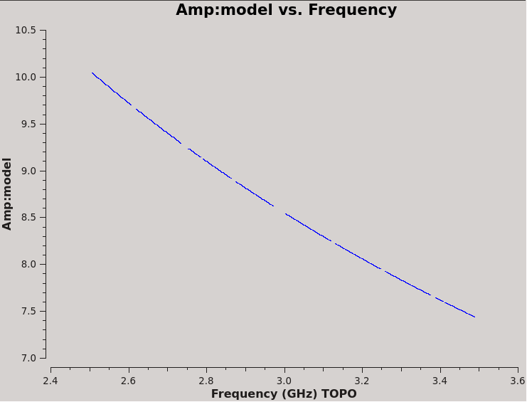
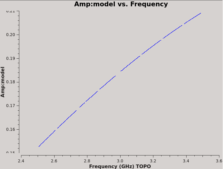
We can see the results in the model column in plotms (Figure 5A) showing the model source spectrum:
# In CASA
plotms(vis='TDRW0001_calibrated.ms',field='0',correlation='RR',
       timerange='',antenna='ea01&ea02',
       xaxis='frequency',yaxis='amp',ydatacolumn='model')
We can see this translates to the spectrum in QU (Figure 5B):
# In CASA
plotms(vis='TDRW0001_calibrated.ms',field='0',correlation='RL',
       timerange='',antenna='ea01&ea02',
       xaxis='frequency',yaxis='amp',ydatacolumn='model')
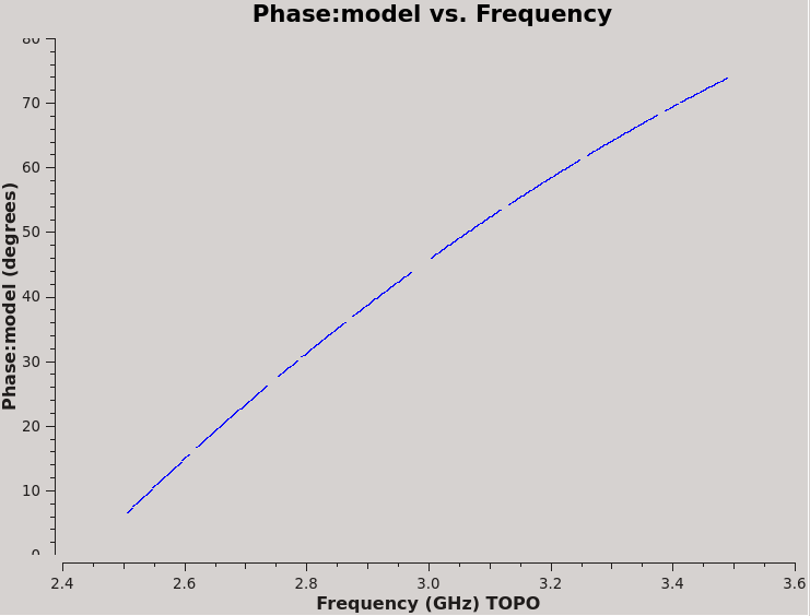
Finally, we plot our R-L phase differences, which should be twice the value of the polarization angle without other complications such as the [math]\displaystyle{ N\pi }[/math] ambiguity (Figure 5C):
# In CASA
plotms(vis='TDRW0001_calibrated.ms',field='0',correlation='RL',
       timerange='',antenna='ea01&ea02',
       xaxis='frequency',yaxis='phase',ydatacolumn='model')
 |
 |
 |
In order to obtain the correct amplitude scaling for instrumental polarization calibration, we need to also specify the Stokes I model that was used for the D-term calibrator(s). The model values of the two D-term calibrators can be obtained from the pipeline weblog under the task hifv_fluxboot inside the CASA log associated with that task. Take this opportunity to try to find them. We've purposely removed the setjy calls in the log so as to not spoil the fun. While not specific to polarization calibration, this exercise should reveal an important aspect of the VLA pipeline: It sets a correct Stokes I model of the secondary calibrators before the final calibration tables are produced (you may appreciate this difference more if you also participated in the Continuum Tutorial and remember how it handled the flux density scale calibration for the secondary calibrators). Your goal when looking over the log is to figure out where the pipeline is getting the inputs for setjy from. Once you've found the relevant lines in the log try to make up the setjy calls on your own.
2023-01-03 19:07:54	INFO	fluxscale::::	 Fitted spectrum for J2355+4950 with fitorder=2: Flux density = 1.76871 +/- 0.000646066 (freq=2.98457 GHz) spidx: a_1 (spectral index) =-0.599569 +/- 0.00275835 a_2=-0.196812 +/- 0.0670986 covariance matrix for the fit:  covar(0,0)=8.14129e-08 covar(0,1)=-1.12826e-07 covar(0,2)=-2.46336e-05 covar(1,0)=-1.12826e-07 covar(1,1)=2.4614e-05 covar(1,2)=0.000242613 covar(2,0)=-2.46336e-05 covar(2,1)=0.000242613 covar(2,2)=0.0145649

2023-01-03 19:07:55	INFO	fluxscale::::	 Fitted spectrum for J0259+0747 with fitorder=2: Flux density = 0.970568 +/- 0.000712514 (freq=2.98457 GHz) spidx: a_1 (spectral index) =0.169919 +/- 0.00510126 a_2=-0.143294 +/- 0.134104 covariance matrix for the fit:  covar(0,0)=1.87159e-06 covar(0,1)=-2.56746e-06 covar(0,2)=-0.000583154 covar(1,0)=-2.56746e-06 covar(1,1)=0.000479139 covar(1,2)=-9.51772e-05 covar(2,0)=-0.000583154 covar(2,1)=-9.51772e-05 covar(2,2)=0.331122
This translates to the following setjy calls.
setjy(vis='TDRW0001_calibrated.ms',
      field='J2355+4950',
      spw='',
      selectdata=False,
      timerange="",
      scan="",
      intent="",
      observation="",
      scalebychan=True,
      standard="manual",
      model="",
      modimage="",
      listmodels=False,
      fluxdensity=[1.76871, 0, 0, 0],
      spix=[-0.599569, -0.196812],
      reffreq="2.98457GHz",
      polindex=[],
      polangle=[],
      rotmeas=0,
      fluxdict={},
      useephemdir=False,
      interpolation="nearest",
      usescratch=True,
      ismms=False,
)

setjy(vis='TDRW0001_calibrated.ms',
      field='J0259+0747',
      spw='',
      selectdata=False,
      timerange="",
      scan="",
      intent="",
      observation="",
      scalebychan=True,
      standard="manual",
      model="",
      modimage="",
      listmodels=False,
      fluxdensity=[0.970568, 0, 0, 0],
      spix=[0.169919, -0.143294],
      reffreq='2.98457GHz',
      polindex=[],
      polangle=[],
      rotmeas=0,
      fluxdict={},
      useephemdir=False,
      interpolation="nearest",
      usescratch=True,
      ismms=False,
)
Solving for the Cross-Hand delays
Just as the pipeline did for the parallel-hand (RR,LL) delays before bandpass calibration, we solve for the cross-hand (RL,LR) delays because of the residual delay difference between the R and L on the reference antenna used for the original delay calibration (ea10 in this tutorial). In our case we simply use 3C48, which has a moderately polarized signal in the RL,LR correlations, and we set its polarized model above using setjy. Since the release of CASA 6.1.2, there are two options to solve for the cross-hand delays, both of them will be illustrated here. The first option fits the cross-hand delay for the entire baseband (here 8 spectral windows form a single baseband), which we call multiband delay. The second option solves the cross-hand delay independently per spectral window. Note that if a dataset contains multiple basebands and you wanted to solve for multiband delays, gaincal has to be executed for each baseband separately, selecting the appropriate spectral windows and appending the results to a single calibration table for later use.
# In CASA

# Solve using Multiband Delay
kcross_mbd = "TDRW0001_calibrated.Kcross_mbd"
gaincal(vis='TDRW0001_calibrated.ms',
    caltable=kcross_mbd,
    field='0137+331=3C48',
    spw='0~7:5~58',
    refant='ea10',
    gaintype="KCROSS",
    solint="inf",
    combine="scan,<?>",
    calmode="ap",
    append=False,
    gaintable=[''],
    gainfield=[''],
    interp=[''],
    spwmap=[[]],
    parang=True)

# Solve using Single Band Delay
kcross_sbd = "TDRW0001_calibrated.Kcross_sbd"
gaincal(vis='TDRW0001_calibrated.ms',
    caltable=kcross_sbd,
    field='0137+331=3C48',
    spw='0~7:5~58',
    refant='ea10',
    gaintype="KCROSS",
    solint="inf",
    combine="scan",
    calmode="ap",
    append=False,
    gaintable=[''],
    gainfield=[''],
    interp=[''],
    spwmap=[[]],
    parang=True)
These commands essentially only differ with how the 'combine' parameter is defined. Based on the description above what should this parameter be in order to fit across the entire baseband?
The only real difference between the commands is that the first is using the entire baseband as input to create one solution and the second is using each spectral window to get individual solutions. In order to tell CASA to combine all of the spectral windows (and scans in this case) one simply has to use: combine='scan,spw'.
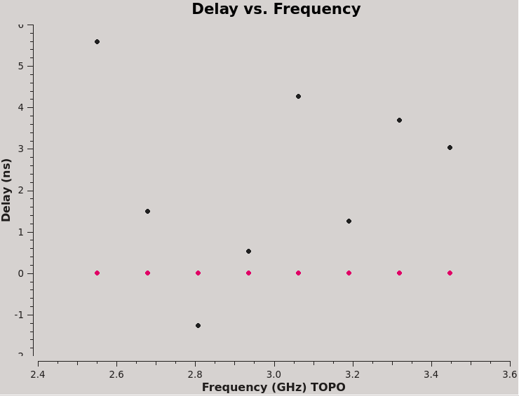
We can plot the single band solutions (see Figure 6):
# In CASA
plotms(vis=kcross_sbd,xaxis='frequency',yaxis='delay',antenna='ea10',coloraxis='corr')
You can also look at the solutions reported in the logger.
For multiband delay there is one solution:
Multi-band cross-hand delay=3.68373 nsec

For single band delay there are 8 solutions:
Spw=0 Global cross-hand delay=5.58964 nsec
Spw=1 Global cross-hand delay=1.49907 nsec
Spw=2 Global cross-hand delay=-1.26208 nsec
Spw=3 Global cross-hand delay=0.522402 nsec
Spw=4 Global cross-hand delay=4.25883 nsec
Spw=5 Global cross-hand delay=1.25194 nsec
Spw=6 Global cross-hand delay=3.69895 nsec
Spw=7 Global cross-hand delay=3.02677 nsec
Notice that the per spectral window solutions are very scattered. The mean delay is 2.32 ns, quite different from the multiband delay. This demonstrates the strength of fitting the cross-hand delay across multiple spectral windows, especially when using a calibrator with a significant frequency dependence, i.e. rotation measure and a polarization fraction of only a few percent. We will continue calibration using the single multiband delay that was derived at 3.68 ns.
Solving for the Leakage Terms
The task polcal is used for polarization calibration. In this data set, we observed the unpolarized calibrator J2355+4950 to demonstrate solving for the instrumental polarization. Task polcal uses the Stokes I, Q, and U values in the model data (Q and U being zero for an unpolarized calibrator) to derive the leakage solutions. We also observed the polarized calibrator J0259+0747 (which has about 4.7% fractional polarization) that is also our complex gain calibrator.
# In CASA

# J2355+4950 / Df
dtab_J2355 = 'TDRW0001_calibrated.Df'
polcal(vis='TDRW0001_calibrated.ms',
       caltable=dtab_J2355,
       field='J2355+4950',
       spw='0~7',
       refant='ea10',
       poltype='Df',
       solint='inf,2MHz',
       combine='scan',
       gaintable=[kcross_mbd],
       gainfield=[''],
       spwmap=[[0,0,0,0,0,0,0,0]],
       append=False)

# J0259+0747 / Df+QU
dtab_J0259 = 'TDRW0001_calibrated.DfQU'
polcal(vis='TDRW0001_calibrated.ms',
       caltable=dtab_J0259,
       intent='CALIBRATE_POL_LEAKAGE#UNSPECIFIED',
       spw='0~7',
       refant='ea10',
       poltype='Df+QU',
       solint='inf,2MHz',
       combine='scan',
       gaintable=[kcross_mbd],
       gainfield=[''],
       spwmap=[[0,0,0,0,0,0,0,0]],
       append=False)
- caltable : polcal will create a new calibration table containing the leakage solutions, which we specify with the caltable parameter.
- field= or intent= : The unpolarized source J2355+4950 is used to solve for the leakage terms in the unpolarized case. For the polarized source J0259+0747 we set the intent leakage polarization.
- spw='0~7' : Select all spectral windows.
- poltype='Df' or poltype='Df+QU' : Solve for the leakages (D) on a per-channel basis (f), assuming zero source polarization, +QU will also solve for the calibrator polarization Q,U per spectral window.
- solint='inf,2MHz', combine='scan' : One solution over the entire run, per spectral channel of 2 MHz
- gaintable=['kcross_mbd']: The previous Kcross multiband delay is applied
- spwmap=[0,0,0,0,0,0,0,0]: This applies a spectral window map, where the first spw solution in the kcross_mbd table is mapped to all other spectral windows. Note there is only one value listed inside the kcross calibration table which is for the lowest spectral window that was used when solving using the multiband delay option (i.e. combine='spw' ).
In the case of Df+QU, the logger window will show the Q/U values it derived for the calibrator and the corresponding polarization fraction and angle that can be derived.
Fractional polarization solution for J0259+0747 (spw = 0): : Q = 0.0259049, U = 0.0336301  (P = 0.0424505, X = 26.1967 deg)
Fractional polarization solution for J0259+0747 (spw = 1): : Q = 0.0139972, U = 0.0382244  (P = 0.0407066, X = 34.944 deg)
Fractional polarization solution for J0259+0747 (spw = 2): : Q = 0.0165052, U = 0.0384224  (P = 0.0418175, X = 33.3765 deg)
Fractional polarization solution for J0259+0747 (spw = 3): : Q = 0.0118274, U = 0.0422875  (P = 0.0439104, X = 37.1871 deg)
Fractional polarization solution for J0259+0747 (spw = 4): : Q = 0.00816816, U = 0.0404744  (P = 0.0412903, X = 39.2952 deg)
Fractional polarization solution for J0259+0747 (spw = 5): : Q = 0.00649365, U = 0.0412879  (P = 0.0417954, X = 40.5309 deg)
Fractional polarization solution for J0259+0747 (spw = 6): : Q = -0.00225595, U = 0.0429258  (P = 0.0429851, X = 46.5042 deg)
Fractional polarization solution for J0259+0747 (spw = 7): : Q = -0.00776873, U = 0.0474773  (P = 0.0481087, X = 49.6465 deg)
From this you can see that J0259+0747 has a fractional polarization of 4.1–4.8% across the 1 GHz bandwidth with a small rotation measure causing a change in angle from 26 to 49 degrees over 1 GHz. In cases where the derived Q/U values seem random and the fractional polarization seems to be very small you might be able to derive better D-term solutions by using poltype='Df' .
After we run the two executions of polcal, you are strongly advised to examine the solutions with plotms to ensure that everything looks good and to compare the results using two different calibrators and poltype methods.
# In CASA
plotms(vis=dtab_J0259,xaxis='freq',yaxis='amp',
       iteraxis='antenna',coloraxis='corr')

plotms(vis=dtab_J2355,xaxis='freq',yaxis='amp',
       iteraxis='antenna',coloraxis='corr')

plotms(vis=dtab_J0259,xaxis='chan',yaxis='phase',
       iteraxis='antenna',coloraxis='corr',plotrange=[-1,-1,-180,180])

plotms(vis=dtab_J2355,xaxis='chan',yaxis='phase',
       iteraxis='antenna',coloraxis='corr',plotrange=[-1,-1,-180,180])
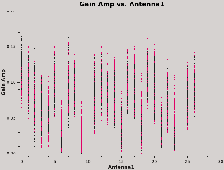
This will produce plots similar to those shown in Figures 7A-D. You can cycle through the antennas by clicking the Next button within plotms. You should see leakages of between 5–17% in most cases. Both Df and Df+QU results should be comparable. However, we will be using the solutions from J0259+0747 to continue calibration and will use J2355+4950 to verify the polarization calibration.
We can also display these in a single plot versus antenna index (see Figure 8):
# In CASA
plotms(vis=dtab_J0259,xaxis='antenna1',yaxis='amp',coloraxis='corr')
Solving for the R-L polarization angle
Having calibrated for the instrumental polarization, the total polarization is now correct, but the R-L phase still needs to be calibrated in order to obtain an accurate polarization position angle. We use the same task, polcal, but this time set parameter poltype='Xf', which specifies a frequency-dependent (f) position angle (X) calibration using the source 3C48, the position angle of which is known, having set this earlier with setjy. Note that we must correct for the leakages before determining the R-L phase, which we do by adding the calibration table made in the previous step (dtab_J0259) to the kcross table that is applied on-the-fly.
# In CASA
xtab = "TDRW0001_calibrated.Xf"
polcal(vis='TDRW0001_calibrated.ms',
       caltable=xtab,
       spw='0~7',
       field='0137+331=3C48',
       solint='inf,2MHz',
       combine='scan',
       poltype='Xf',
       refant = 'ea10',
       gaintable=[kcross_mbd,dtab_J0259],
       gainfield=['',''],
       spwmap=[[0,0,0,0,0,0,0,0],[]],
       append=False)
Strictly speaking, there is no need to specify a reference antenna for poltype='Xf' (for circularly polarized receivers only) because the X solutions adjust the cross-hand phases for each antenna to match the given polarization angle of the model. However, for consistency/safety, it is recommended to always specify refant when performing polarization calibration.
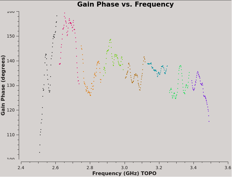
It is strongly suggested you check that the calibration worked properly by plotting up the newly-generated calibration table using plotms (see Figure 9):
# In CASA
plotms(vis=xtab,xaxis='frequency',yaxis='phase',coloraxis='spw')
Because the Xf term captures the residual R-L phase on the reference antenna over the array, there is only one value for all antennas. Also, as we took out the RL delays using the Kcross solution, these Xf variations do not show a significant slope in phase. And since we were using a single multiband delay, the phases connect from one spectral window to another; had we used the single band delays, we would see phase jumps from one to another spectral window.
At this point, you have all the necessary polarization calibration tables.
Applying the Calibration
Now that we have derived all the calibration solutions, we need to apply them to the actual data using the task applycal. The measurement set DATA column contains the original split data. To apply the calibration we have derived, we specify the appropriate calibration tables which are then applied to the DATA column, with the results being written in the CORRECTED_DATA column.
# In CASA
applycal(vis = 'TDRW0001_calibrated.ms',
         field='',
         gainfield=['', '', ''],
         flagbackup=True,
         interp=['', '', ''],
         gaintable=[kcross_mbd,dtab_J0259,xtab],
         spw='0~7',
         calwt=[False, False, False],
         applymode='calflagstrict',
         antenna='*&*',
         spwmap=[[0,0,0,0,0,0,0,0],[],[]],
         parang=True)
- gaintable : We provide a Python list of the calibration tables to be applied. This list must contain the cross-hand delays (kcross), the leakage calibration (dtab; here derived from J0259+0747), and the R-L phase corrections (xtab).
- calwt=[False] : At the time of this writing, we are not yet using system calibration data to compute real (1/Jy2) weights; trying to calibrate them can produce nonsensical results. Experience has shown that calibrating the weights will lead to problems, especially in the self-calibration steps. You can specify calwt on a per-table basis, here is set all to False.
- parang : If polarization calibration has been performed, set parameter parang=True.
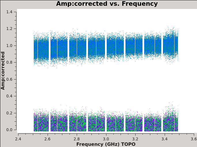
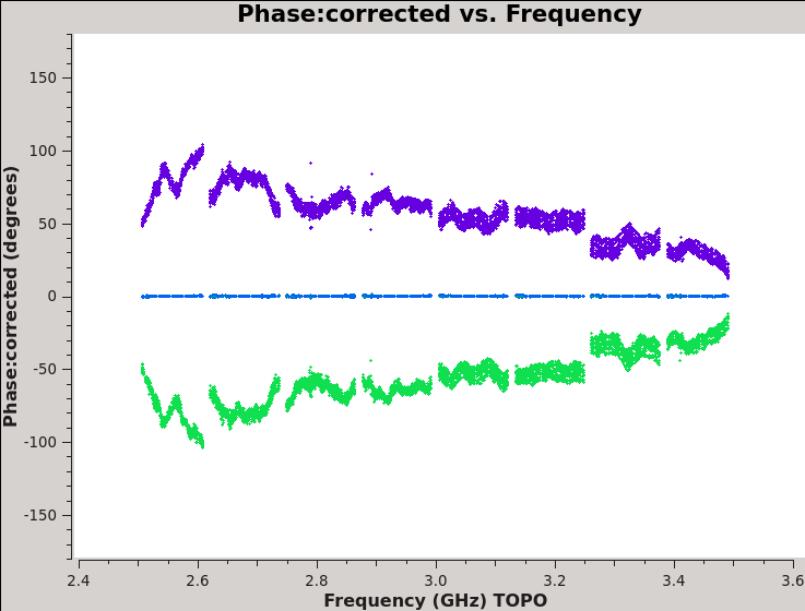
We should now have fully-calibrated visibilities in the CORRECTED_DATA column of the measurement set, and it is worthwhile pausing to inspect them to ensure that the calibration did what we expected it to. We make some standard plots (see Figures 10A-F). Now that you've used plotms a few times try making the below plots on your own. The only bit of information you cannot derive from the figures themselves is that we have averaged them in time by 60 seconds.
# In CASA
plotms(vis='TDRW0001_calibrated.ms',field='0',correlation='',
       timerange='',antenna='',avgtime='60',
       xaxis='frequency',yaxis='amp',ydatacolumn='corrected',
       coloraxis='corr',
       plotfile='Plotms-3C48-fld0-corrected-amp-CASA6.4.1.jpeg')

plotms(vis='TDRW0001_calibrated.ms',field='0',correlation='',
       timerange='',antenna='',avgtime='60',
       xaxis='frequency',yaxis='phase',ydatacolumn='corrected',
       plotrange=[-1,-1,-180,180],coloraxis='corr',
       plotfile='Plotms-3C48-fld0-corrected-phase-CASA6.4.1.jpeg')

plotms(vis='TDRW0001_calibrated.ms',field='1',correlation='',
       timerange='',antenna='',avgtime='60',
       xaxis='frequency',yaxis='amp',ydatacolumn='corrected',
       coloraxis='corr',
       plotfile='Plotms-J2355-fld1-corrected-amp-CASA6.4.1.jpeg')

plotms(vis='TDRW0001_calibrated.ms',field='1',correlation='RR,LL',
       timerange='',antenna='',avgtime='60',
       xaxis='frequency',yaxis='phase',ydatacolumn='corrected',
       plotrange=[-1,-1,-180,180],coloraxis='corr',
       plotfile='Plotms-J2355-fld1-corrected-phase-CASA6.4.1.jpeg')

plotms(vis='TDRW0001_calibrated.ms',field='2',correlation='',
       timerange='',antenna='',avgtime='60',
       xaxis='frequency',yaxis='amp',ydatacolumn='corrected',
       coloraxis='corr',
       plotfile='Plotms-J0259-fld2-corrected-amp-CASA6.4.1.jpeg')

plotms(vis='TDRW0001_calibrated.ms',field='2',correlation='',
       timerange='',antenna='',avgtime='60',
       xaxis='frequency',yaxis='phase',ydatacolumn='corrected',
       plotrange=[-1,-1,-180,180],coloraxis='corr',avgbaseline=True,
       plotfile='Plotms-J0259-fld2-corrected-phase-CASA6.4.1.jpeg')
For 3C48 (figures 10A, 10B) we see the polarized signal in the cross-hands; there is some sign of bad data remaining in 3C48. Also, the RL phase plots of J0259+4950 (figure 10F) indicate that the Xf solutions, thus polarization angles, in the lowest two spectral windows are problematic. You can also estimate from the RL,LR amplitudes in J2355+4950 (figure 10E) what the level of residual instrumental polarization, which we expect to be around <0.5%. A more accurate evaluation of residual instrumental polarization fraction can be made imaging the secondary D-term calibrator per spectral window and calculating its residual polarization.
 |
 |
Now that the calibration has been applied to the target data, we split off the science targets to create a new, calibrated measurement set containing the target field.
# In CASA
split(vis='TDRW0001_calibrated.ms',outputvis='3C75.ms',
      datacolumn='corrected',field='3')
- outputvis : We give the name of the new measurement set to be written, which will contain the calibrated data on the science target.
- datacolumn : We use the CORRECTED_DATA column, containing the calibrated data which we just wrote using applycal.
- field : We wish to place the target field into a measurement set for imaging and joint deconvolution.
Prior to imaging, it is a good idea to run the statwt task to correct the data weights (weight and sigma columns) in the measurement set. Running statwt will remove the effects of relative noise scatter that may have been introduced from flagging uneven bits in the visibility data between the channels and times. We will run this task here on the newly calibrated and split data set before moving on to imaging.
# In CASA
statwt(vis='3C75.ms',datacolumn='data',minsamp=8)
Imaging
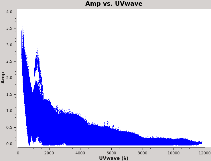
Now that we have split off the target data into a separate measurement set with all the calibration applied, it's time to make an image. It is important to have an idea of what values to use for the image pixel (cell) size and the overall size of the image. Setting the appropriate pixel size for imaging depends upon basic optics aspects of interferometry. Use plotms to look at the newly calibrated, target-only data set:
# In CASA
plotms(vis='3C75.ms',xaxis='uvwave',yaxis='amp',
       ydatacolumn='data', field='0',avgtime='30',correlation='RR',
       plotfile='plotms_3c75-uvwave.jpeg',avgspw=False,overwrite=True)
You should obtain a plot similar to Figure 11 with the (calibrated) visibility amplitude as a function of [math]\displaystyle{ u }[/math]-[math]\displaystyle{ v }[/math] distance. You will also see some outliers there which are primarily from residual amplitude errors of ea05, that had a warm receiver which we can isolate to particular time periods. We will be addressing this after the initial imaging.
Based on the UVwave plot can you determine approximately what the smallest angular scale of the image will be?
We can see in the plot that the maximum baseline is about 12,000 wavelengths. If we recall that the VLA works via diffraction then it follows that: [math]\displaystyle{ \theta\approx\lambda/D=1/12000 radians\approx17 arcsec }[/math]. Furthermore, the most effective cleaning occurs with 3–5 pixels across the synthesized beam. So for this data a cell size of 3.4 arcseconds will give just about 5 pixels per beam.
The 3C75 binary black hole system is known to have a maximum extent of at least 8-9 arcminutes, corresponding to about 147 pixels for the chosen cell size. Therefore, we need to choose an image size that covers most of the extent of the source. We therefore set imsize=[480,480] and the source will fit comfortably within that image.
In this tutorial, we will run tclean interactively so that we can set and modify the mask:
# In CASA
tclean(vis='3C75.ms',
       field="3C75",
       spw="",timerange="",
       uvrange="",antenna="",scan="",observation="",intent="",
       datacolumn="data",
       imagename="3C75_initial",
       imsize=480,
       cell="3.4arcsec",
       phasecenter="",
       stokes="IQUV",
       projection="SIN",
       specmode="mfs",
       reffreq="3.0GHz",
       nchan=-1,
       start="",
       width="",
       outframe="LSRK",
       veltype="radio",
       restfreq=[],
       interpolation="linear",
       gridder="standard",
       mosweight=True,
       cfcache="",
       computepastep=360.0,
       rotatepastep=360.0,
       pblimit=0.0001,
       normtype="flatnoise",
       deconvolver="mtmfs",
       scales=[0, 6, 18],
       nterms=2,
       smallscalebias=0.6,
       restoration=True,
       restoringbeam=[],
       pbcor=False,
       outlierfile="",
       weighting="briggs",
       robust=0.5,
       npixels=0,
       uvtaper=[],
       niter=20000,
       gain=0.1,
       threshold=0.0,
       nsigma=0.0,
       cycleniter=1000,
       cyclefactor=1.0,
       restart=True,
       savemodel="modelcolumn",
       calcres=True,
       calcpsf=True,
       parallel=False,
       interactive=True)
Task tclean is powerful with many inputs and a certain amount of experimentation likely is required. The below is an explanation of several of the parameters we've used.
- vis='3C75.ms' : this split MS contains the target field only.
- imagename='3C75_initial' : our output image cubes will all start with this name root, e.g., 3C75_initial.image
- specmode='mfs' : Use multi-frequency synthesis imaging. The fractional bandwidth of these data is non-zero (1000 MHz at a central frequency of 3.0 GHz). Recall that the [math]\displaystyle{ u }[/math] and [math]\displaystyle{ v }[/math] coordinates are defined as the baseline coordinates, measured in wavelengths. Thus, slight changes in the frequency from channel to channel result in slight changes in [math]\displaystyle{ u }[/math] and [math]\displaystyle{ v }[/math]. There is a concomitant improvement in [math]\displaystyle{ u }[/math]-[math]\displaystyle{ v }[/math] coverage if the visibility data from the multiple spectral channels are gridded separately onto the [math]\displaystyle{ u }[/math]-[math]\displaystyle{ v }[/math] plane, as opposed to treating all spectral channels as having the same frequency.
- niter=20000,gain=0.1,threshold='0.0mJy' : Recall that the gain is the amount by which a clean component is subtracted during the cleaning process. Parameters niter and threshold are (coupled) means of determining when to stop the cleaning process, with niter specifying to find and subtract that many clean components while threshold specifies a minimum flux density threshold a clean component can have before tclean stops (also see interactive below). Imaging is an iterative process, and to set the threshold and number of iterations, it is usually wise to clean interactively in the first instance, stopping when spurious emission from sidelobes (arising from gain errors) dominates the residual emission in the field. Here, we have set the threshold level to zero and let the tclean task define an appropriate threshold. The number of iterations should then be set high enough to reach the threshold found by tclean.
- gridder='standard' : The standard tclean gridder is sufficient for our purposes, since we are not combining multiple pointings from a mosaic or try to perform widefield imaging in an extended configuration.
- interactive=True : Very often, particularly when one is exploring how a source appears for the first time, it can be valuable to interact with the cleaning process. If True, interactive causes a viewer window to appear. One can then set clean regions, restricting where tclean searches for clean components, as well as monitor the cleaning process. A standard procedure is to set a large value for niter, and stop the cleaning when it visually appears to be approaching the noise level. This procedure also allows one to change the cleaning region, in cases when low-level intensity becomes visible as the cleaning process proceeds.
- imsize=480,cell='3.4arcsec' : See the discussion above regarding setting the image size and cell size. If only one value is specified for the parameter, the same value is used in both directions (declination and right ascension).
- stokes='IQUV' : tclean will output an image cube containing all: total intensity I, and Stokes Q, U, and V.
- deconvolver='mtmfs', scales=[0, 6, 18], smallscalebias=0.9 : The settings for scales are in units of pixels, with 0 pixels equivalent to the traditional delta-function clean. The scales here are chosen to provide delta functions and then two logarithmically scaled sizes to fit to the data. The first scale (6 pixels) is chosen to be comparable to the size of the synthesized beam. The smallscalebias attempts to balance the weight given to larger scales, which often have more flux density, and the smaller scales, which often are brighter. Considerable experimentation is likely to be necessary; one of the authors of this document found that it was useful to clean several rounds with this setting, change to multiscale=[] and remove much of the smaller scale structure, then return to this setting.
- weighting='briggs',robust=0.5 : 3C75 has diffuse, extended emission that is, at least partially, resolved out by the interferometer even though we are in the most compact VLA configuration. A naturally-weighted image would show large-scale patchiness in the noise. In order to suppress this effect, Briggs weighting is used (intermediate between natural and uniform weighting), with a default robust factor of 0.5 (which corresponds to something between natural and uniform weighting).
- pbcor=False : by default pbcor=False and a flat-noise image is produced. We can do the primary beam correction later (see below).
- savemodel='modelcolumn' : We recommend here the use of a physical MODEL_DATA scratch column. This will save some time, as it can be faster in the case of complicated gridding to read data from disk instead of doing all of the computations on-the-fly. However, this has the unfortunate side effect of increasing the size of the MS on disk.
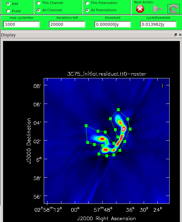
As mentioned above, we can guide the clean process by allowing it to find clean components only within a user-specified region. When tclean runs in interactive mode, an imview window will pop up as shown in Figure 12. First, you'll want to navigate to the green box and select "All Polarizations" rather than use the default "This Polarization"; this way the cleaning we are about to do will apply to all of the polarizations rather than just the one we are currently viewing. Similarly, select "All channels". To get a more detailed view of the central regions containing the emission, zoom in by first left clicking on the zoom button (leftmost button in third row) and tracing out a rectangle with the left mouse button and double-clicking inside the zoom box you just made. Play with the color scale to bring out the emission better by holding down the middle mouse button and moving it around. To create a clean box (a region within which components may be found), hold down the right mouse button and trace out a rectangle around the source, then double-click inside that rectangle to set it as a box. Note that the clean box must turn white for it to be registered - if the box is not white, it has not been set. Alternatively, you can trace out a more custom shape to better enclose the irregular outline of the radio galaxy jets. To do this, right-click on the closed polygonal icon then trace out a shape by right-clicking where you want the corners of that shape. Once you have come full circle, the shape will be traced out in green, with small squares at the corners. Double-click inside this region and the green outline will turn white. You have now set the clean region. If you have made a mistake with your clean box, click on the Erase button, trace out a rectangle around your erroneous region, and double-click inside that rectangle. You can also set multiple clean regions.
At any stage in the cleaning, you can adjust the number of iterations that tclean will do before returning to the GUI (cycleniter). This is set to 1000 (see the iterations field in mid-upper left of panel), values from 500 to 1000 later on seem to work. Note that this will override the cycleniter value that you might had set before starting tclean. tclean will keep going until it reaches threshold or runs out of cycles (the cycles field to the right of the iterations).
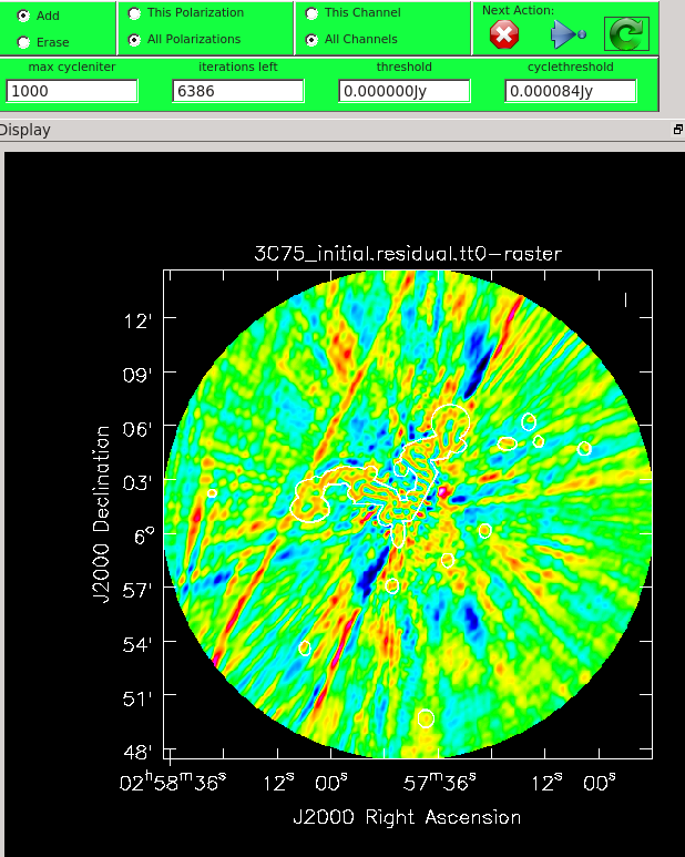
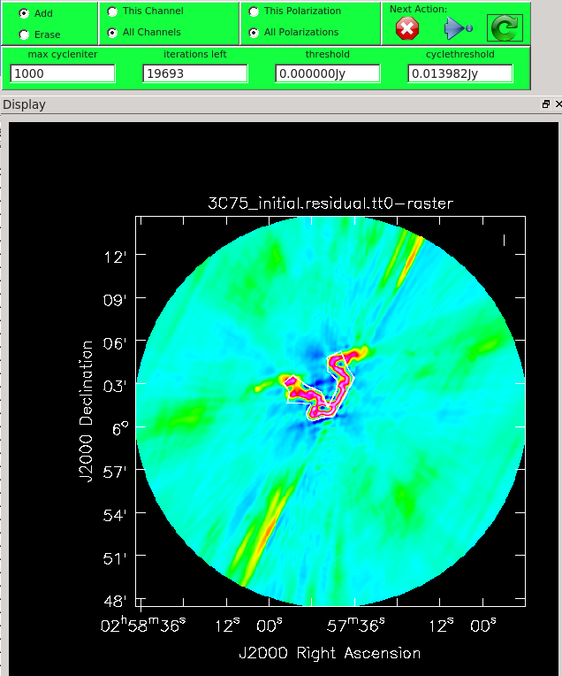
When you are happy with the clean regions, press the green circular arrow button on the far right to continue deconvolution. After completing a cycle, a revised image will come up. As the brightest points are removed from the image (cleaned off), fainter emission may show up. You can adjust the clean boxes each cycle, to enclose all real emission. After many cycles, when only noise is left, you can hit the red-and-white stop-sign icon to stop cleaning. Figure 13 shows the interactive viewer panel later in the process, after cleaning about 500 iterations. We have used the polygon tool to add to the clean region, drawing around emission that shows up in the residual image outside of the original clean region. After about 13000 iterations (Figure 14) the residuals were looking good (similar noise level inside and outside of the cleaned mask region). As mentioned before, restarting tclean with different multiscale=[...] choices can help also. You see that there is a significant amount of residual structure (the various spikes and streaks throughout the image), these are most likely due to calibration errors which we will try to correct for in the next section during self-calibration.
Task tclean will make several output files, all named with the prefix given as imagename. These include:
- .image: final restored image(s) with the clean components convolved with a restoring beam and added to the remaining residuals at the end of the imaging process, one for each Taylor Term (.tt0 and .tt1)
- .pb.tt0: effective response of the telescope (the primary beam)
- .mask: areas where tclean has been allowed to search for emission
- .model: sum of all the clean components, which also has been stored as the MODEL_DATA column in the measurement set, one for each Taylor Term (.tt0 and .tt1)
- .psf: dirty beam, which is being deconvolved from the true sky brightness during the clean process, one for each Taylor Term (.tt0, .tt1, .tt2)
- .residual: what is left at the end of the deconvolution process; this is useful to diagnose whether or not to clean more deeply, one for each Taylor Term (.tt0, .tt1)
- .sumwt: a single pixel image containing sum of weights per plane, one for each Taylor Term (.tt0, .tt1, .tt2)
After the imaging and deconvolution process has finished, you can use CARTA to look at your image.
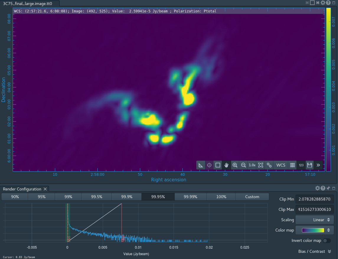
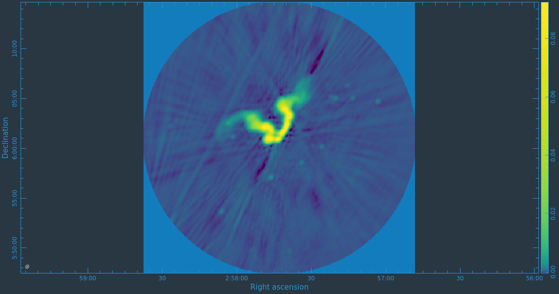
Take some time to play with the color scale to better emphasize the faint emission and to see the underlying noise patterns. For the figures above we selected the viridis color map, the linear scale function, and the 99.9% data range on the histogram. You can also use the Animators slider/buttons to switch between the four different Stokes parameter images that were computed. If you are unfamiliar with CARTA then take some time to look over its extensive built in documentation and help features. You can find its searchable online manual via the "Help" button at the top or to get more information on a particular widget you can click the corresponding "?" button near it. If you click the Animator tab you'll also notice that CARTA attempts to create total polarization, linear polarization, fractional total polarization, fractional linear polarization, and linear polarization angle images for you. This can be quite convenient, but we'll show how to create these yourself later in this guide.
The tclean task naturally operates in a flat noise image, i.e., an image where the effective weighting across the field of view is set so that the noise is constant. This is so that the clean threshold has a uniform meaning for the stopping criterion and that the image fed into the minor cycles has uniform noise levels. This means, however, that the image does not take into account the primary beam response fall-off in the edges. In principle, tclean produces primary beam response image, and if we had set parameter pbcor=True tclean would had saved a primary beam corrected restored image of our target. Since we used deconvolver='mtmfs' and nterms=2, the calculation of the primary beam response requires special treatment. To perform wideband primary beam correction, we will use task widebandpbcor. In the future this task will be incorporated into tclean, but until then this separate task needs to be used.
# In CASA
widebandpbcor(vis='3C75.ms',imagename='3C75_initial',nterms=2, action='pbcor',
              spwlist=[0,1,2,3,4,5,6,7], chanlist=[32,32,32,32,32,32,32,32], weightlist=[1,1,1,1,1,1,1,1])
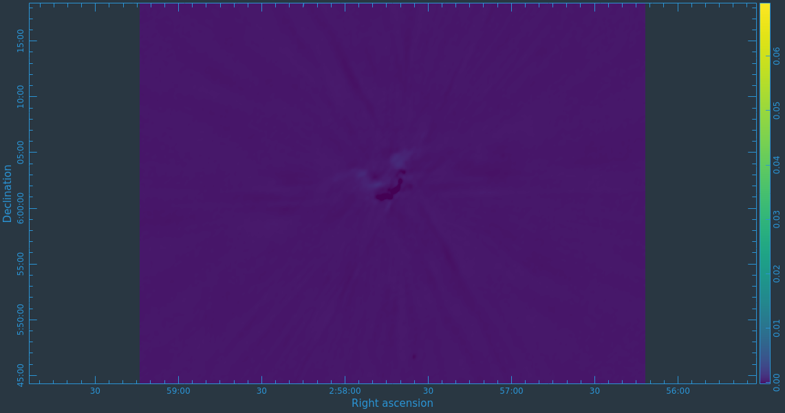
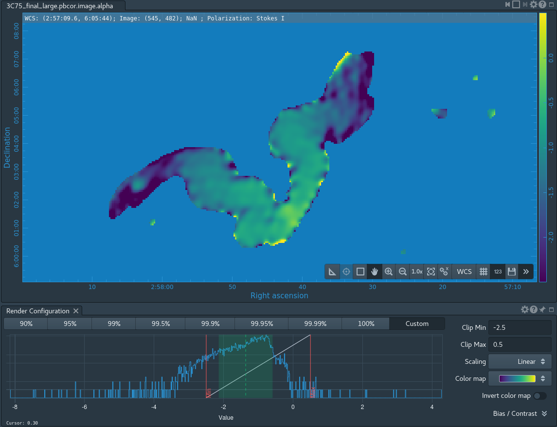
The task will produce primary beam corrected images of our target (3C75_initial.pbcor.image.tt0, 3C75_initial.pbcor.image.tt1, 3C75_initial.pbcor.image.alpha, 3C75_initial.pbcor.image.alpha.error). You can open image 3C75_initial.pbcor.image.tt0 in CARTA, and compare it to screenshots in Figure 15. You will see noise (and signal) at the edges of the image has indeed increased.
Self-Calibration
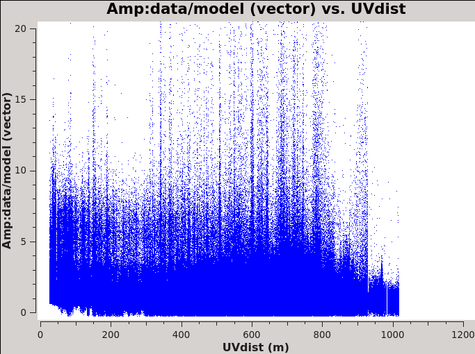
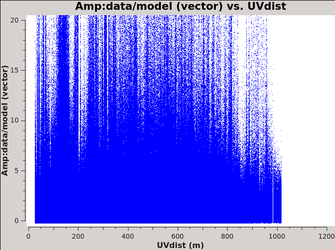
Before we get started with self-calibration, it might be good to check whether we need to perform additional flagging on the target data. Since we have established an image model in the previous section, we can use it to look at the residuals by dividing out the model. We can make a similar plot to Figure 11 above, however, we will divide the image model that was created. The division will help us to see low level interfrence we might not otherwise notice by just looking at the data column. Since we performed full-polarization imaging, we can also do the same to the cross-hand data RL,LR. Figures 16A & B shows example plots. You should also have a look at time plotted against amplitude and frequency against amplitude to see if there are any obvious times of interference.
# In CASA
plotms(vis='3C75.ms',xaxis='uvdist',yaxis='amp',plotrange=[0,0,0,20],
       ydatacolumn='data/model_vector', field='3C75',avgtime='30',correlation='RR',
       plotfile='plotms_3c75-uvdist_resid_RR.png',avgspw=False,overwrite=True)

# If you made a mistake above and didn't clean the polarization as well, then this plot will be empty.
plotms(vis='3C75.ms',xaxis='uvdist',yaxis='amp',plotrange=[0,0,0,20],
       ydatacolumn='data/model_vector', field='3C75',avgtime='30',correlation='RL',
       plotfile='plotms_3c75-uvdist_resid_RL.png',avgspw=False,overwrite=True)
Since we are seeing a significant amount of weak residual interference, we will take a few steps to reduce these.
# In CASA

# tfcrop
flagdata(vis='3C75.ms',mode='tfcrop',correlation='ABS_RR,ABS_LL',freqfit='line',extendflags=False,flagbackup=False,datacolumn='residual_data',flagdimension='freq',ntime='scan')
flagdata(vis='3C75.ms',mode='tfcrop',correlation='ABS_RL,ABS_LR',freqfit='line',extendflags=False,flagbackup=False,datacolumn='residual_data',flagdimension='freq',ntime='scan')
# rflag
flagdata(vis='3C75.ms',mode='rflag',correlation='RR,LL',extendflags=False,flagbackup=False,datacolumn='residual_data',ntime='scan')
flagdata(vis='3C75.ms',mode='rflag',correlation='RL,LR',extendflags=False,flagbackup=False,datacolumn='residual_data',ntime='scan')
# extend flags
flagdata(vis='3C75.ms',mode='extend',flagbackup=False)
This should have gotten rid of the worst remaining outliers, but will leave some residual weak RFI on certain baseline lengths. Since we are not trying to win any records on high dynamic range imaging, this additional flagging should suffice for our dataset.
In addition to residual RFI, even after calibration using the amplitude calibrator and the phase calibrator, there are likely to be residual phase and/or amplitude errors in the data. Self-calibration uses an existing model, often constructed from imaging the data itself, provided that sufficient visibility data have been obtained. This is essentially always the case with data: the system of equations is wildly over-constrained for the number of unknowns.
For an array of [math]\displaystyle{ N }[/math] antennas there are at any given instant only [math]\displaystyle{ N }[/math] gain factors, but how many visibilities?
[math]\displaystyle{ {N(N-1) \over 2} }[/math]
Since we are only considering one instance of time (i.e. one integration) this is also the number of baselines in the array. For a typical 27 antenna VLA observation that comes out to 351.
For an array with a reasonable number of antennas, [math]\displaystyle{ N }[/math] >~ 8, solutions to this set of coupled equations converge quickly. There is some discussion in the old CASA Reference Manual on self calibration (see Section 5.11), but more detailed discussion can be found in lectures on Self-calibration given at NRAO community days.
In self-calibrating data, it is useful to keep in mind the structure of a Measurement Set. There are three columns of interest for an MS: the DATA column, the MODEL column, and the CORRECTED_DATA column. In normal usage, as part of the initial split, the DATA column of the new MS is set to be equal the previous MS's CORRECTED_DATA column. The self-calibration procedure is then:
- Produce an image (tclean) using the (corrected copy) DATA column.
- Derive a series of gain corrections (gaincal) by comparing the DATA columns and the Fourier transform of the image, which is stored in the MODEL column. These corrections are stored in an external table.
- Optionally, we can also derive a bandpass correction—which is also referred to as bandpass self calibration—to correct for global amplitude errors.
- Apply these corrections (applycal) to the DATA column to form a new CORRECTED_DATA column overwriting the previous contents of CORRECTED_DATA should it exist.
The following example begins with the standard data set, 3C75.ms (resulting from the steps above). We have previously generated an IQUV multiscale image cube. We discard it for this step and create a new Stokes I image, which we will use to generate a series of gain corrections (phase only self-calibration) that will be stored in 3C75.ScG0. With this solution, we then perform bandpass self-calibration to remove any amplitude slope that might be present. Next, we apply the derived phase and amplitude corrections to the data to form a set of self-calibrated data, and then re-image the dataset (3C75_selfcal.image). For the purpose of self-calibration, note that in the clean before the self-calibration, it is important that we only use the Stokes I model so that any cleaned polarization does not affect the gaincal. We first use delmod on the MS to get rid of the previous polarized model, and run tclean to generate Stokes I-only image.
#In CASA
delmod('3C75.ms')

tclean(vis='3C75.ms',
       field="3C75",
       spw="",timerange="",
       uvrange="",antenna="",scan="",observation="",intent="",
       datacolumn="data",
       imagename="3C75_initial_I",
       imsize=480,
       cell="3.4arcsec",
       phasecenter="",
       stokes="I",
       projection="SIN",
       specmode="mfs",
       reffreq="3.0GHz",
       nchan=-1,
       start="",
       width="",
       outframe="LSRK",
       veltype="radio",
       restfreq=[],
       interpolation="linear",
       gridder="standard",
       mosweight=True,
       cfcache="",
       computepastep=360.0,
       rotatepastep=360.0,
       pblimit=0.0001,
       normtype="flatnoise",
       deconvolver="mtmfs",
       scales=[0, 6, 18],
       nterms=2,
       smallscalebias=0.6,
       restoration=True,
       restoringbeam=[],
       pbcor=False,
       outlierfile="",
       weighting="briggs",
       robust=0.5,
       npixels=0,
       uvtaper=[],
       niter=3500,
       gain=0.1,
       threshold=0.0,
       nsigma=0.0,
       cycleniter=750,
       cyclefactor=1.0,
       restart=True,
       savemodel="modelcolumn",
       calcres=True,
       calcpsf=True,
       parallel=False,
       interactive=True)
As discussed, this tclean call will ignore the polarized structure. You should not clean very deeply at this point. You want to be sure to capture as much of the source's total flux density as possible, but not include low level questionable features or sub-structures (ripples) that might be due to calibration or deconvolution artifacts. We modified the two parameters controlling tclean's minor and major cycles to the following values cycleniter=750 and niter=3500 to reflect this, but you may find that you don't even need 3500 iterations for this first tclean pass.
If you are happy with the new image, perform the following self-calibration steps:
#In CASA
gaincal(vis='3C75.ms', caltable='3C75.ScG0', field='', solint='inf', refant='ea10',
           spw='',minsnr=3.0, gaintype='G', parang=False, calmode='p')

bandpass(vis='3C75.ms', caltable='3C75.ScB0', field='', solint='inf', refant='ea10', minsnr=3.0, spw='',
                parang = False, gaintable=['3C75.ScG0'], interp=[])

applycal(vis='3C75.ms', gaintable=['3C75.ScG0','3C75.ScB0'], spw='', applymode='calflagstrict', parang=False)
The CORRECTED_DATA column of the MS now contains the self-calibrated visibilities which will be used by next execution of tclean. The gaincal step will report a number of solutions with insufficient SNR. By default, with parameter applymode='calflag', data with no good solutions will be flagged by applycal which may or may not be a good thing. You can control the action of applycal by changing the value of parameter applymode. Setting applymode='calflagstrict' will be more stringent about flagging data points without valid calibration, while applymode='calonly' will calibrate those with solutions while passing unchanged the data without solutions. You can see ahead of time what applycal will do by executing it with applymode='trial' which will do the reporting but nothing else. In our example we used applymode='calflagstrict' , but you will notice that the reported flagged fraction has not changed much, only increasing by 0.6%. This is a good thing.
Having applied these gain and bandpass solutions, we will once again image the target measurement set which we now expect to have better gain solutions and consequently produce a better image. We do this by invoking the tclean command once again.
#In CASA
tclean(vis='3C75.ms',
       field="3C75",
       spw="",timerange="",
       uvrange="",antenna="",scan="",observation="",intent="",
       datacolumn="corrected",
       imagename="3C75_selfcal_1",
       imsize=480,
       cell="3.4arcsec",
       phasecenter="",
       stokes="I",
       projection="SIN",
       specmode="mfs",
       reffreq="3.0GHz",
       nchan=-1,
       start="",
       width="",
       outframe="LSRK",
       veltype="radio",
       restfreq=[],
       interpolation="linear",
       gridder="standard",
       mosweight=True,
       cfcache="",
       computepastep=360.0,
       rotatepastep=360.0,
       pblimit=0.0001,
       normtype="flatnoise",
       deconvolver="mtmfs",
       scales=[0, 6, 18],
       nterms=2,
       smallscalebias=0.6,
       restoration=True,
       restoringbeam=[],
       pbcor=False,
       outlierfile="",
       weighting="briggs",
       robust=0.5,
       npixels=0,
       uvtaper=[],
       niter=3500,
       gain=0.1,
       threshold=0.0,
       nsigma=0.0,
       cycleniter=750,
       cyclefactor=1.0,
       restart=True,
       savemodel="modelcolumn",
       calcres=True,
       calcpsf=True,
       parallel=False,
       interactive=True)
Commonly this self-calibration procedure is applied multiple times. In Figures 17A & B you can see a comparison of the shallow Stokes I image before self-calibration and after two self-calibration steps. The first self-calibration round was done as instructed in this section, while the second round was executed with solint='120s' and new solution tables were created (3C75.ScG1, 3C75.ScB1). You are encouraged to think about what parameters should and should not differ between the round 1 and round 2 self calibration stages, but they are provided below.
#In CASA
gaincal(vis='3C75.ms', caltable='3C75.ScG1', field='', solint='120s', refant='ea10',
           spw='',minsnr=3.0, gaintype='G', parang=False, calmode='p')

bandpass(vis='3C75.ms', caltable='3C75.ScB1', field='', solint='inf', refant='ea10', minsnr=3.0, spw='',
                parang = False, gaintable=['3C75.ScG1'], interp=[])

applycal(vis='3C75.ms', gaintable=['3C75.ScG1','3C75.ScB1'], spw='', applymode='calflagstrict', parang=False)

#Producing the Figure 17B image
tclean(vis='3C75.ms',
       field="3C75",
       spw="",timerange="",
       uvrange="",antenna="",scan="",observation="",intent="",
       datacolumn="corrected",
       imagename="3C75_selfcal_2",
       imsize=480,
       cell="3.4arcsec",
       phasecenter="",
       stokes="I",
       projection="SIN",
       specmode="mfs",
       reffreq="3.0GHz",
       nchan=-1,
       start="",
       width="",
       outframe="LSRK",
       veltype="radio",
       restfreq=[],
       interpolation="linear",
       gridder="standard",
       mosweight=True,
       cfcache="",
       computepastep=360.0,
       rotatepastep=360.0,
       pblimit=0.0001,
       normtype="flatnoise",
       deconvolver="mtmfs",
       scales=[0, 6, 18],
       nterms=2,
       smallscalebias=0.6,
       restoration=True,
       restoringbeam=[],
       pbcor=False,
       outlierfile="",
       weighting="briggs",
       robust=0.5,
       npixels=0,
       uvtaper=[],
       niter=3500,
       gain=0.1,
       threshold=0.0,
       nsigma=0.0,
       cycleniter=750,
       cyclefactor=1.0,
       restart=True,
       savemodel="modelcolumn",
       calcres=True,
       calcpsf=True,
       parallel=False,
       interactive=True)
Note that only the gaincal call used the 120s solint. The bandpass of the VLA antennas are generally stable in time so it is relatively rare to have a case for using a time variable bandpass. Also note that the new solution interval is not the only difference between these round 2 calls. Since our previous tclean call (imagename="3C75_selfcal_1") also used savemodel='modelcolumn' these calls will be making use of an improved model.
 |
 |
The number of iterations is determined by a combination of the data quality, the number of antennas in the array, the structure of the source, the extent to which the original self-calibration assumptions are valid, and the user's patience. A not uncommon limitation for moderately high dynamic range imaging is that there may be baseline-based factors that modify the true visibility. If the corruptions to the true visibility cannot be modeled as antenna-based self-calibration won't help.
Self-calibration requires experimentation. Do not be afraid to remove an image, or even a set of gain corrections, change something and try again. Having said that, here are several guidelines to consider:
- Bookkeeping is important! Suppose one conducts 9 iterations of self-calibration. Will it be possible to remember one month later (or maybe even one week later!) which set of gain corrections and images are which? In the example above, the descriptor 'selfcal_1' is attached to various files to help keep straight what is what. Successive iterations of self-cal could then be 'selfcal_2' , 'selfcal_3' , etc.
- Care is required in setting imagename. If one has an image that already exists, CASA will continue cleaning it (if it can), which is almost certainly not what one wants during self-calibration. Rather, use a unique imagename for each pass of self-calibration.
- A common metric for self-calibration is whether the dynamic range (= peak flux density/rms) of the image has improved. An improvement of 10% is quite acceptable.
- Be careful when making images and setting clean regions or masks; self-calibration assumes that the model is perfect. If one cleans a noise bump, self-calibration will quite happily try to adjust the gains so that the CORRECTED_DATA describe a source at the location of the noise bump. It is far better to exclude some features of a source, or a weak source, from initial cleaning and conduct another round of self-calibration than to create an artificial source. If a real source is excluded from initial cleaning, it will continue to be present in subsequent iterations of self-calibration; if it's not a real source, one probably isn't interested in it anyway.
- Start self-calibration with phase-only solutions (parameter calmode='p' in gaincal). As discussed in the High Dynamic Range Imaging lecture, a phase error of 20 deg is as bad as an amplitude error of 10%.
- In initial rounds of self-calibration, consider solution intervals longer than the nominal sampling time (parameter solint in gaincal) and/or lower signal-to-noise ratio thresholds (parameter minsnr in gaincal). Depending upon the frequency and configuration and fidelity of the model image, it can be quite reasonable to start with solint='30s' or solint='60s' and/or minsnr=3. One may also want to consider specifying a uvrange, if, for example, the field has structure on large scales (small [math]\displaystyle{ u }[/math]-[math]\displaystyle{ v }[/math]) that is not well represented by the current image.
- The task applycal will flag data with no good calibration solutions. During the initial self-calibration steps, this flagging may be excessive. If so, one can restore the flags to the state right before running applycal by using the task flagmanager.
- You can track the agreement between the DATA, CORRECTED_DATA, and MODEL in plotms. The options in Axes tab allows one to select which column is to be plotted. If the MODEL agrees well with the CORRECTED_DATA, one can use shorter solint and/or higher minsnr values.
- You should consider examining the solutions from gaincal by using plotms in order to assure that the corrections are sensible. Smoothly varying phases are good, jumps are usually not. (However, because the phases are often plotted ±180 degrees, there can be apparent jumps if the phases are very near +180 deg or −180 deg.)
Final Polarization Images
At this point, satisfied with the results of self-calibration, it might be a good idea to recalculate the visibility weights since some additional flagging was performed. After this, we get right to full-polarization imaging. We also suspect that there is a bright source outside of the masked field causing some imaging artifacts due to not being cleaned. We thus set the parameter pbmask value to 0.0 in order to disable masking of areas beyond the primary beam, and make the image larger to incorporate the bright source into our model in this tclean execution.
# In CASA
statwt(vis='3C75.ms', minsamp=8, datacolumn='corrected', flagbackup=True)

tclean(vis='3C75.ms',
       field="3C75",
       spw="",timerange="",
       uvrange="",antenna="",scan="",observation="",intent="",
       datacolumn="corrected",
       imagename="3C75_final_large",
       imsize=800,
       cell="3.4arcsec",
       phasecenter="",
       stokes="IQUV",
       projection="SIN",
       specmode="mfs",
       reffreq="3.0GHz",
       nchan=-1,
       start="",
       width="",
       outframe="LSRK",
       veltype="radio",
       restfreq=[],
       interpolation="linear",
       gridder="standard",
       mosweight=True,
       cfcache="",
       computepastep=360.0,
       rotatepastep=360.0,
       pblimit=-0.0001,
       pbmask=0.0,
       normtype="flatnoise",
       deconvolver="mtmfs",
       scales=[0, 6, 18],
       nterms=2,
       smallscalebias=0.6,
       restoration=True,
       restoringbeam=[],
       pbcor=False,
       outlierfile="",
       weighting="briggs",
       robust=0.5,
       npixels=0,
       uvtaper=[],
       niter=20000,
       gain=0.1,
       threshold=0.0,
       nsigma=0.0,
       cycleniter=1000,
       cyclefactor=1.0,
       restart=True,
       savemodel="modelcolumn",
       calcres=True,
       calcpsf=True,
       parallel=False,
       interactive=True)
The final restored Stokes I,Q,U, and V images are shown in Figures 18A–D. We've set the color scale to match between the images. Note that there is still a star like pattern in the residuals which are artifacts most likely due to the multi-scale multi-term multi-frequency synthesis. You can try on your own to improve upon the shown images by re-imaging and choosing a different set of multi-scale parameters that better match the scales found in the extended structure of 3C 75. Another issue to point out is looking at the Stokes V image. We do not expect a significant amount of Stokes V emission from this object, the emission you are seeing in Stokes V is most likely an effect of incorrectly solving for polarization leakages in the primary beam. In the above calibration we have only addressed leakage between the two polarization referring to the phase center. The extended beam itself, however, shows leakage which manifests itself spatially. The extended polarized emission we see in the Stokes Q and U images is not corrected for beam polarization during imaging. This, in turn, contains errors leading to polarization and de-polarization effects and causes changes to the polarization angle which increases the further away one gets from the beam center. Additionally, the two polarization beams do not sit on top of each other but are slightly offset, introducing a polarization squint. For correct and accurate polarization imaging, these two effects have to be taken into account. Imaging algorithms to address beam polarization are currently under development and will be discussed in this guide when they become available to the general user.
Note, that these images are not yet primary beam corrected and are displayed on log scaling. You should play with the color scaling as well as the bias/contrast widget in CARTA to better see the faint emission.
Spectral & Polarization Maps
Note: If you are using CARTA then several of the next steps are actually unnecessary. If supplied a proper IQUV image CARTA will compute polarization intensity, linear polarization, fractional polarization intensity, fractional linear polarization intensity, and polarization angle maps for you. We show the steps one would have to take to manually create some of the images below for completeness. When possible the Figures shown will be using values/images that are generated soley by CARTA itself. You are encouraged though to still manually create your own set of images and then overlay them with the CARTA generated images to see that they match.
If you want to obtain a reasonable map of the in-band spectral index, like the one shown in Fig. 19A, we can compute it with the task widebandpbcor. As demonstrated earlier, the task can also correct the images for the telescope's primary beam response; this correction will make the images science ready. Parameter action='pbcor' will perform both actions (correct for the primary beam and calculate spectral index map) while parameter threshold sets minimum flux density above which the spectral index is calculated (this will allow us to mask all the noise regions).
# In CASA
widebandpbcor(vis='3C75.ms', imagename='3C75_final_large', nterms=2, threshold='1.0mJy/beam', action='pbcor',
              spwlist=[0,1,2,3,4,5,6,7], chanlist=[32,32,32,32,32,32,32,32], weightlist=[1,1,1,1,1,1,1,1])
For further study of polarization properties, you might want to convert the Stokes images into something more useful for scientific analysis. We will use CASA to calculate polarization intensity, [math]\displaystyle{ \sqrt{Q^2 + U^2 + V^2} }[/math], and polarization angle, [math]\displaystyle{ {atan2 (U,Q) \over 2} }[/math], maps from the final Stokes I,Q,U,V images. You can then look at those with CARTA. For example, Figure 19B shows the polarization intensity image. Since we've yet to apply any mask, the polarization angle image made in the next step will also contain values from low signal-to-noise data.
# In CASA

# Obtain image for the polarization intensity
immath(outfile='3C75_final.poli',mode='poli',imagename=['3C75_final_large.image.tt0'],sigma='0.0Jy/beam')
# Obtain image for the polarization angle
immath(outfile='3C75_final.pola',mode='pola',imagename=['3C75_final_large.image.tt0'],sigma='0.0Jy/beam')
Note that for calculations of the polarization intensity and angle images you may — but do not need to — use primary beam corrected images; your results will be the same. This is because the primary beam correction cancels out in the equations for these two polarization quantities. If you want to visualize the polarization vectors on top of the Stokes I image, we need to add a mask for the low noise values.
# In CASA
!cp -r '3C75_final.poli' polimg

imsubimage(imagename='3C75_final_large.image.tt0',outfile='3C75_final.Q.image',stokes='Q')
imsubimage(imagename='3C75_final_large.image.tt0',outfile='3C75_final.U.image',stokes='U')

subimPI='polimg'
ia.open(subimPI)
ia.calcmask(mask=subimPI+'>5e-4',name='mymask')
ia.done()

ia.open('3C75_final.Q.image')
ia.maskhandler('copy',['polimg:mymask','polithreshmask'])
ia.maskhandler('set','polithreshmask')
ia.done()

ia.open('3C75_final.U.image')
ia.maskhandler('copy',['polimg:mymask','polithreshmask'])
ia.maskhandler('set','polithreshmask')
ia.done()

immath(imagename=['3C75_final.Q.image', '3C75_final.U.image'], mode='pola', outfile='3C75_final.pola.masked')
These steps take the polarized intensity image calculated above (Figure 19B) and create a mask using a polarization intensity threshold of 5e-4 Jy/beam. This mask is then applied to the Q and U images from the image cube that was generated above. Then a new polarization angle image is calculated from the Q & U image planes, applying the mask created from the polarization intensity image. Finally, we can load the Stokes I as raster image into CARTA and add the polarization angle as vectors. You can do this by matching the final IQUV image, 3C75_final_large.image.tt0, and the newly created polarization angle image in WCS space by clicking the "XY" under the "Matching" column of the Image List widget. Then open the Vector Overlay Configuration widget to create the vectors. You can compare the vectors calculated with immath to the ones that CARTA generates for you. You may notice that there are some vectors that appear to disagree with each other. If so, it is likely caused by the pixel averaging being done within CARTA, which you can toggle off to confirm. Figure 19C shows the resulting image. One can clearly see that the linear polarization angle follows perpendicular to the extended structure. This indicates that the magnetic field lines are oriented along the extended structure, perpendicular to the linear polarization angles.
Rotation Measures
The plane of polarization of light is rotated by the magnetic fields present in the intervening plasma. The total rotation to the plane of polarization of light between the source and the user is called Faraday Rotation. Prior to the wide bandwidth capabilities, these rotation measures were computed by fitting a line to the polarization position angle as a function of the square of the wavelength of measurement. The slope of the resulting fit was deemed to be the RM of the source while the intercept would give the true polarization position angle of the source. With the wide bandwidths, it is now possible to determine the rotation measure of the source using the naive fitting approach by making images per spectral window in IQUV and fitting the data (polarization position angle vs lambda^2) with a line.
We show how to produce such images with one last tclean call using the following parameters. Since this is the last tclean call you'll need to perform to complete the guide we'll give you the opportunity to see if you can construct it yourself (Tip: using 'inp tclean' in CASA to see the inputs for the command will be quite useful). Remember two key differences in this call as compared to the previous:
- You are making a cube with one spectral window per plane
- You already know where the emission is (i.e. you have a mask)
# In CASA
tclean(vis='3C75.ms',
       field="3C75",
       spw="",timerange="",
       uvrange="",antenna="",scan="",observation="",intent="",
       datacolumn="corrected",
       imagename="3C75_chan8",
       imsize=800,
       cell="3.4arcsec",
       phasecenter="",
       stokes="IQUV",
       projection="SIN",
       specmode="cube",
       reffreq="",
       nchan=-1,
       start="",
       width=64,
       outframe="LSRK",
       veltype="radio",
       restfreq=[],
       interpolation="linear",
       gridder="standard",
       mosweight=True,
       cfcache="",
       computepastep=360.0,
       rotatepastep=360.0,
       pblimit=-0.0001,
       pbmask=0.0,
       mask='3C75_final_large.mask',
       normtype="flatnoise",
       deconvolver="multiscale",
       scales=[0, 6, 18],
       nterms=1,
       smallscalebias=0.6,
       restoration=True,
       restoringbeam=[],
       pbcor=False,
       outlierfile="",
       weighting="briggs",
       robust=0.5,
       npixels=0,
       uvtaper=[],
       niter=20000,
       gain=0.1,
       threshold=0.0,
       nsigma=0.0,
       cycleniter=1000,
       cyclefactor=1.0,
       restart=True,
       savemodel="none",
       calcres=True,
       calcpsf=True,
       parallel=False,
       interactive=False)
Here's the differences as compared to the previous tclean:
- specmode="cube": This tells tclean we want a cube (i.e. separate images for separate frequencies) instead of a continuum image (specmode='mfs')
- width=64: This tells tclean how wide in number of channels (i.e. frequency) each plane of the cube should be. We wanted one plane per spectral window and our spectral windows are 64 channels wide each.
- mask='3C75_final_large.mask': We created this in our previous tclean call by interactively drawing it in the GUI. We call it again here to reuse it.
- deconvolver="multiscale": Previously we used 'mtmfs' which stands for Multi-Term (Multi-scale) Multi-Frequency Synthesis. Since we are making per spectral window images this time were are no longer in the wideband regime and therefore drop the multi-frequency aspect.
- nterms=1: Same reasoning as the change in deconvolver. Since we are making per spectral window images we need not worry about the spectral index of each image (i.e. we can assume each spectral window has a flat spectrum).
- savemodel="none": This change is not strictly needed, but since we have no intention of changing our model with this run of tclean it is good form to make sure this is set. It would be a shame to overwrite your model this late into the process only to decide later that you wanted it for some reason.
- interactive=False: Since we already have a mask we are happy with from the previous run there is no use in having tclean's GUI pop up again.
Now we use the CASA toolkit to access data for four pixels in the image cube to visualize and fit the rotation measure.
# In CASA
import matplotlib
# to display
matplotlib.use('TkAgg')
import matplotlib.pyplot as plt
import numpy as np

ia.open('3C75_chan8.image')

# number of channels/frequencies
nunr = 8

tt = ia.getchunk()
nu = np.linspace(2.551e9,3.319e9,num=nunr)
c = 2.99792458e8

Q1 = tt[418,444,1,:nunr]
U1 = tt[418,444,2,:nunr]
Q2 = tt[376,419,1,:nunr]
U2 = tt[376,419,2,:nunr]
Q3 = tt[383,401,1,:nunr]
U3 = tt[383,401,2,:nunr]
Q4 = tt[395,398,1,:nunr]
U4 = tt[395,398,2,:nunr]

chi1 = 0.5*np.arctan2(U1,Q1)
chi2 = 0.5*np.arctan2(U2,Q2)
chi3 = 0.5*np.arctan2(U3,Q3)
chi4 = 0.5*np.arctan2(U4,Q4)

#locate the values that are nan and delete these indices from nu
indx1=np.argwhere(chi1==0)
indx2=np.argwhere(chi2==0)
indx3=np.argwhere(chi3==0)
indx4=np.argwhere(chi4==0)

nu1=np.delete(nu,indx1)
lam1 = c/nu1
lamsq1 = lam1*lam1

nu2=np.delete(nu,indx2)
lam2 = c/nu2
lamsq2 = lam2*lam2

nu3=np.delete(nu,indx3)
lam3 = c/nu3
lamsq3 = lam3*lam3

nu4=np.delete(nu,indx4)
lam4 = c/nu4
lamsq4 = lam4*lam4

#drop the zero values
chi1=np.delete(chi1,indx1)
chi2=np.delete(chi2,indx2)
chi3=np.delete(chi3,indx3)
chi4=np.delete(chi4,indx4)

fit1 = np.polyfit(lamsq1,chi1,1)
fit_fn1 = np.poly1d(fit1)
slope1 = fit1[0]
intercept1 = fit1[1]
fit2 = np.polyfit(lamsq2,chi2,1)
fit_fn2 = np.poly1d(fit2)
slope2 = fit2[0]
intercept2 = fit2[1]
fit3 = np.polyfit(lamsq3,chi3,1)
fit_fn3 = np.poly1d(fit3)
slope3 = fit3[0]
intercept3 = fit3[1]
fit4 = np.polyfit(lamsq4,chi4,1)
fit_fn4 = np.poly1d(fit4)
slope4 = fit4[0]
intercept4 = fit4[1]

plt.figure(1)
plt.title('Overall Title')
plt.subplot(221)
plt.title('Point 1: (418,444)')
plt.xlabel(r'$\lambda^{2}$')
plt.ylabel(r'$\chi1$')
plt.scatter(lamsq1,chi1,color='r')
plt.plot(lamsq1,fit_fn1(lamsq1),'r--',label='$\chi$ = {:.2f}$\lambda^2$ + {:.2f}'.format(slope1,intercept1))
plt.legend(loc=2)

plt.subplot(222)
plt.title('Point 2: (376,419)')
plt.xlabel(r'$\lambda^{2}$')
plt.ylabel(r'$\chi2$')
plt.scatter(lamsq2,chi2,color='b')
plt.plot(lamsq2,fit_fn2(lamsq2),'b--',label='$\chi$ = {:.2f}$\lambda^2$ + {:.2f}'.format(slope2,intercept2))
plt.legend(loc=1)

plt.subplot(223)
plt.title('Point 3: (383,401)')
plt.xlabel(r'$\lambda^{2}$')
plt.ylabel(r'$\chi3$')
plt.scatter(lamsq3,chi3,color='g')
plt.plot(lamsq3,fit_fn3(lamsq3),'g--',label='$\chi$ = {:.2f}$\lambda^2$ + {:.2f}'.format(slope3,intercept3))
plt.legend(loc=3)

plt.subplot(224)
plt.title('Point 4: (395,398)')
plt.xlabel(r'$\lambda^{2}$')
plt.ylabel(r'$\chi4$')
plt.scatter(lamsq4,chi4,color='m')
plt.plot(lamsq4,fit_fn4(lamsq4),'m--',label='$\chi$ = {:.2f}$\lambda^2$ + {:.2f}'.format(slope4,intercept4))
plt.legend(loc=1)
plt.tight_layout()

plt.show()
#Or to save the figure
plt.savefig('3C75_rmscript_8chan4px.png')

ia.close()
The resulting plots are shown in Figure 20A. Alternatively, there exists a CASA task rmfit which does this basic fitting for you while taking into account the [math]\displaystyle{ N \pi }[/math] ambiguity (refer to [3] for more info). The fits using rmfit for our case of 3C 75 by making images per spectral window is shown in Figure 20B. Here we set the maximum acceptable position angle error to 20 degrees. If larger, then no rotation measures are calculated.
# In CASA
rmfit('3C75_chan8.image',rm='3C75_chan8_rm.image',rmerr='3C75_chan8_rm.image.err',maxpaerr=0.35)
 |
 |
The rmfit task has many more options; for example, you are able to provide a foreground rotation measure to subtract.
Now we can compare the rotation measures extracted for the 4 pixels from the 8 channel image cube with the values derived in the rmfit for the same pixels. In most cases the values are more or less comparable.
| Point | RM Lin. Fit. | RM RMFIT |
|---|---|---|
| 1 | -65.46 | -57.29 |
| 2 | 10.41 | 66.62 |
| 3 | -71.71 | -65.14 |
| 4 | -7.30 | -5.07 |
If time allows you can take this even further. As our source is rather bright, we can derive an IQUV image not just per averaged spectral window as we just did, but rather per channel. To achieve this you can change the above tclean parameter width from 64 to 1, which will result in 512 channels spanning all 8 spectral windows. Note when imaging each channel, the edge channels are flagged which results in the PSF being blank for channels sourrounding each spectral window and some of the images being blank. Don't forget to change the imagename parameter when re-running tclean. Due to the increased size of the cube you may find that your machine's avaliable memory struggles to keep up with the new tclean command. If so, then you can reduce the image size to lower the required memory. For our 512 channel cube we reduced the image size from 800x800 to 270x270. If you do reduce the image size as we have then you'll need to make use of imsubimage to first reduce your old image's mask size so it can be used again for your smaller image. Following the same steps as for the 8 channel image cube (adjusting for the new number of channels and new pixel indices for our points of interest), you would then obtain the results shown in Figure 21 where again the polarization position angle as a function of lambda square is shown together with the rmfit image. We can clearly see that the source exhibits complex structure beyond a simple linear fit we performed earlier. This suggests that deriving a single RM would be an oversimplification. We should ideally perform RM Synthesis (https://arxiv.org/pdf/astro-ph/0507349.pdf). At this point in time CASA does not have an RM synthesis task.
