VLA-S-CASA Pipeline-CASA6.2.1
This guide is designed for CASA 6.2.1.
Introduction
When VLA observations are complete, the raw data need to be calibrated and imaged for scientific applications. This is achieved through various steps as explained in the VLA CASA tutorials. The different calibration procedures are also bundled in a general VLA calibration pipeline that is described on the VLA pipeline webpage. The pipeline can also include continuum target imaging.
At NRAO, the calibration portion of the pipeline is executed on every science scheduling block (SB) that the VLA observes successfully. Target imaging is left to the user, who can run either the imaging pipeline steps (cf. the VLA pipeline imaging webpage) or revert to manual imaging as explained in the VLA CASA tutorials. The VLA pipeline webpage describes how to run, modify, and re-execute the VLA pipeline. There are also instructions on how to restore archived pipeline products as well as a list of known issues. In the following material, we provide an example of a VLA pipeline weblog (calibration and imaging), explain the different pipeline stages, and describe some of the diagnostic information and plots. Frequent issues with VLA data, and how to address them with the pipeline are discussed on the Pipeline: Frequent VLA problems page, where signatures and treatment of problematic data are discussed.
The following data are VLA S-band continuum observations of the galaxy 3C75, a bright radio galaxy. The pipeline calibration discussed here can be followed up by polarization calibration and imaging as described in the CASA guide Polarization Calibration based on CASA pipeline (3C75).
The Pipeline Weblog
The pipeline run can be inspected through a weblog that is launched by pointing a web browser to file:///<path to your working directory>/pipelineTIME/html/index.html. Note that we regularly test the weblog on Firefox but less so on other browsers. So if you don't use Firefox, there's a chance that not all items are displayed correctly. Additionally, some browser security features may prevent the weblog from being displayed. The weblog may actually show a warning and a solution in the browser.
The following discussion is based on a weblog that can be viewed through the following link:
Pipeline Weblog
Alternatively, the weblog can be downloaded from https://casa.nrao.edu/Data/EVLA/Pipeline/VLApipe-Sguide-weblog-CASA6.2.1.tar.gz (25 MB)
and extracted via:
# In a Terminal
tar xzvf VLApipe-Sguide-weblog-CASA6.2.1.tar.gz
then point your browser to html/index.html (as of CASA 6.2.1 there can be a security setting in Firefox that needs to be set first; the weblog will prompt you with instructions if this is the case [frequently go to "about:config" in FIrefox and set security.fileuri.strict_origin_policy to false]). Chrome may not show all items properly unless started like Chrome --args --allow-file-access-from-files /path/to/weblog//html/index.html).
At the top of the landing page one can find the items Home (the index.html landing page), By Topic and By Task that provide navigation through the pipeline results.
Home Screen
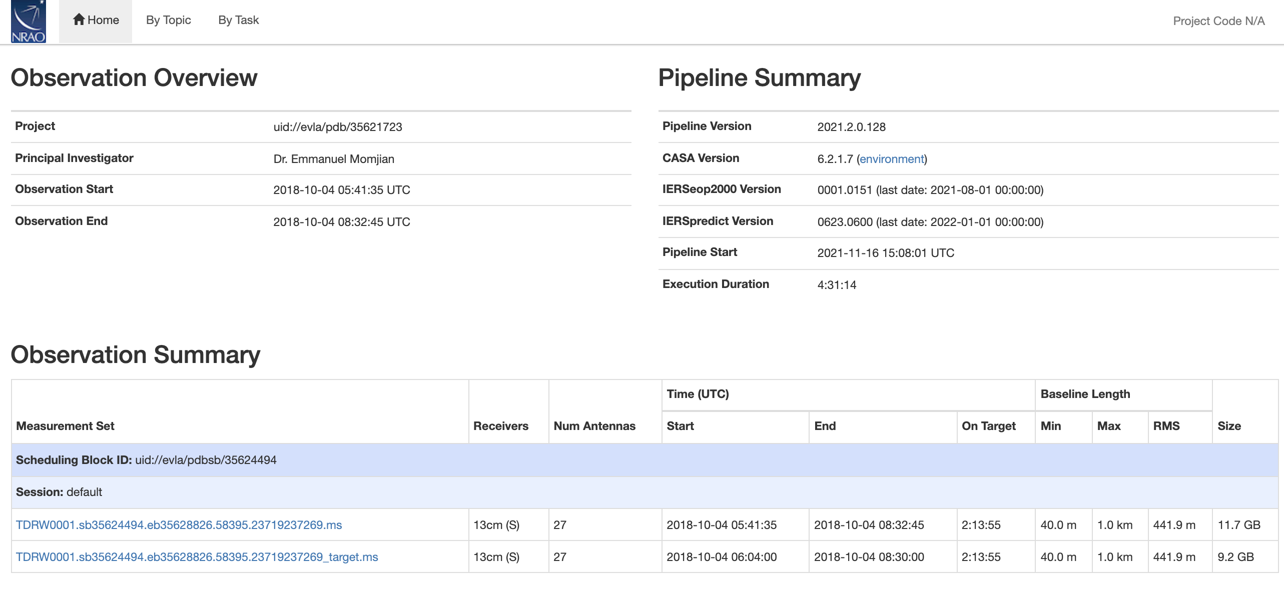
The Home page of the weblog (Fig. 1) contains essential information such as the project archive code, the PI name, and the start and end time of the observations. The CASA and pipeline versions that were used for the pipeline run are also listed on this page, as well as a table with the MS name, receiver bands, number of antennas, on source time, min/max baseline lengths and their rms, and the file size BEFORE CALIBRATION (after processing and adding the MODEL and CORRECTED_DATA columns, the file size triples, as seen in Stage 13: applycals). The data were processed with earth orientation parameters that were available at the time of the processing. The pipeline uses predicted parameters when current ones are not available. The respected file versions for predicted and evaluated earth orientation parameters are listed under "IERSpredict" and "IERSeop2000", as provided by the International Earth Rotation and Reference System Service (IERS). Note that it usually takes a few months until the IERS re-evaluates and publishes updated earth orientation parameters. While the actual numbers of the data products change numerically after obtaining new parameters, the differences for VLA data are usually small and scientifically insignificant.
Since we also include target imaging, the weblog displays two MeasurementSets, the full one used for calibration, and one that only contains the target data.
Overview Screen
An Overview of the observations (Fig. 2) can be obtained by clicking on the MS name. As mentioned above, we look at the first MS, which is the full MS that is used for calibration.
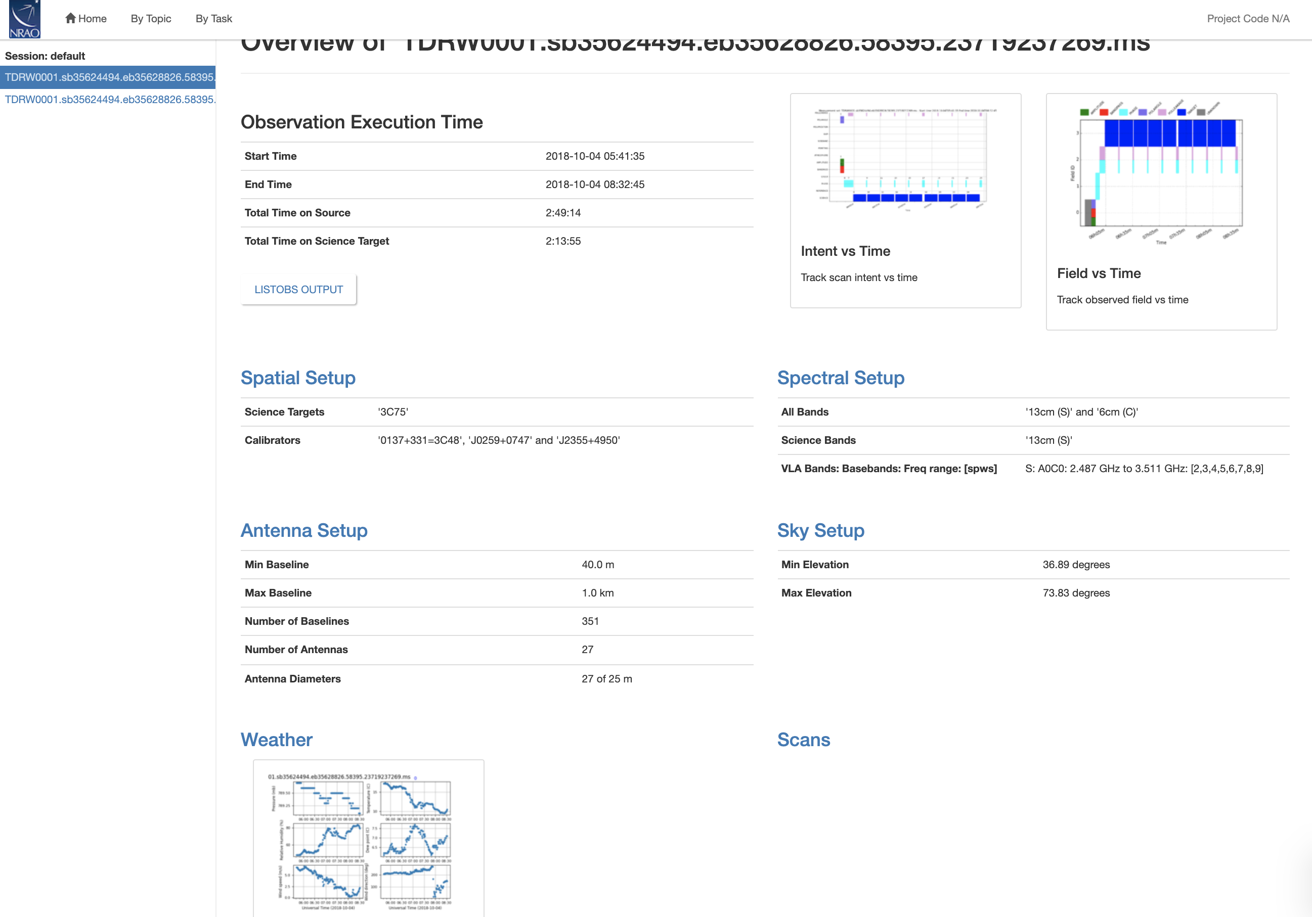
This page provides additional information about the observation. It includes Observation Execution Time (date, time on source in UTC), Spatial Setup (science target and calibrator field names), Antenna Setup (min/max baseline lengths, number of antennas and baselines), Spectral Setup (band designations, including VLA baseband information; science bands include most calibrators, but exclude pointing and setup scans), and Sky Setup (min/max elevation). The page also provides graphical overviews of the scan intent and field ID observing sequence. A plot with weather information is also included. Clicking the blue headers provides additional information on each topic.
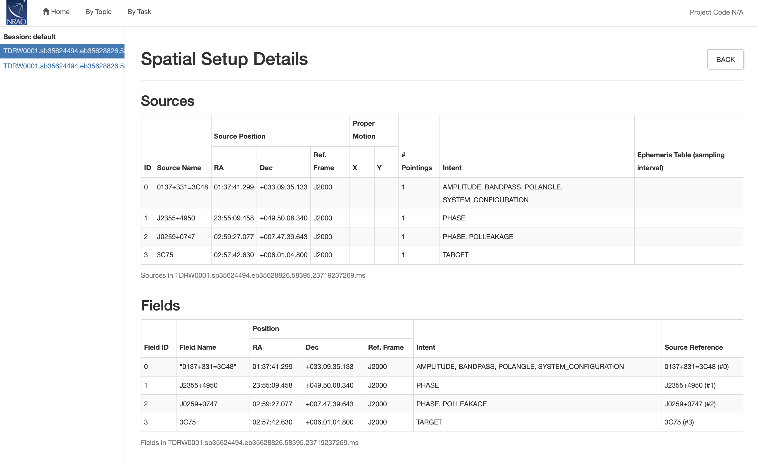
The Spatial Setup page (Fig. 3) lists all sources and fields (where a source is a field with additional information, e.g. it could describe flux variations). Names, IDs, positions, and scan intents are listed for each source/field.
 |
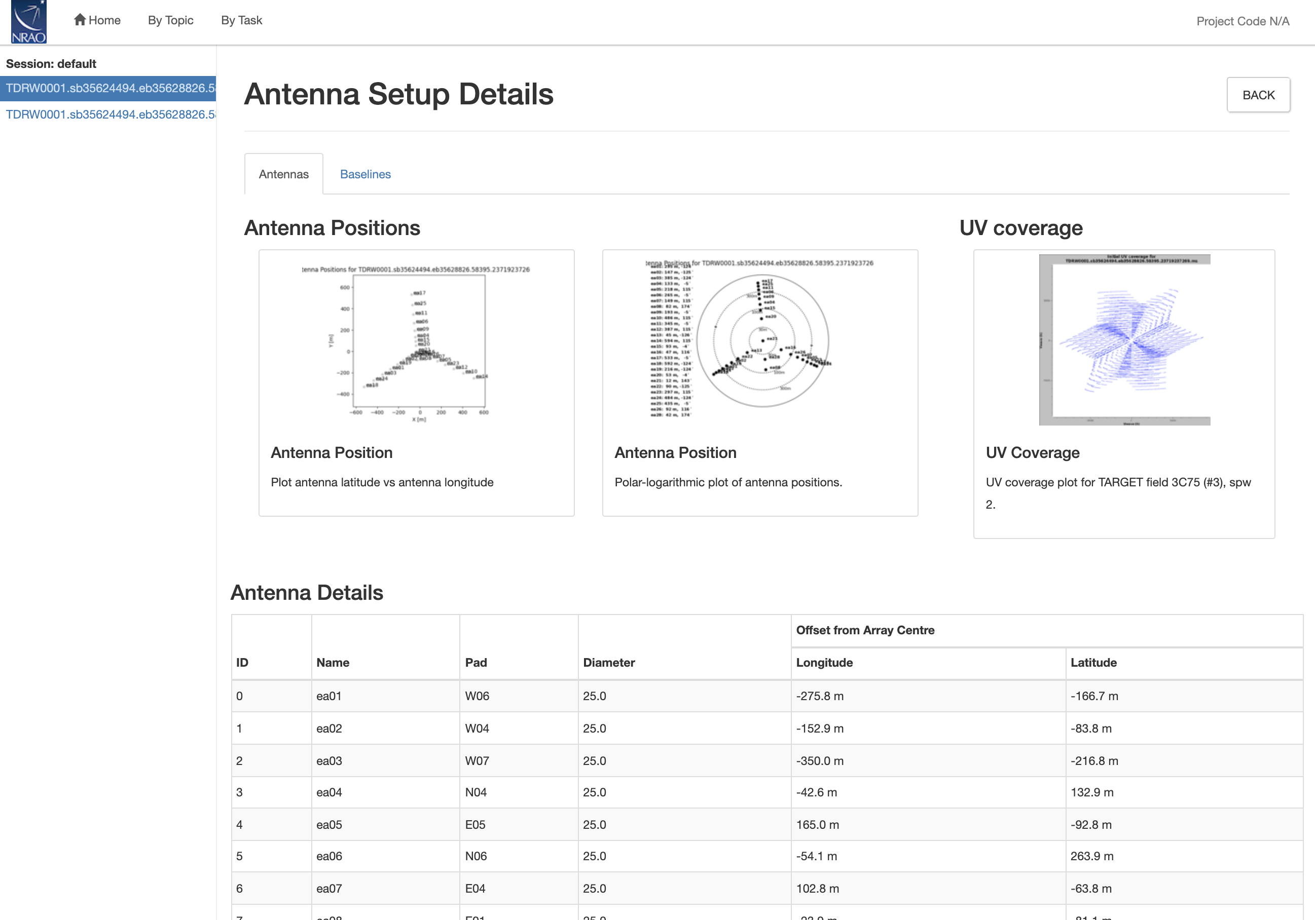
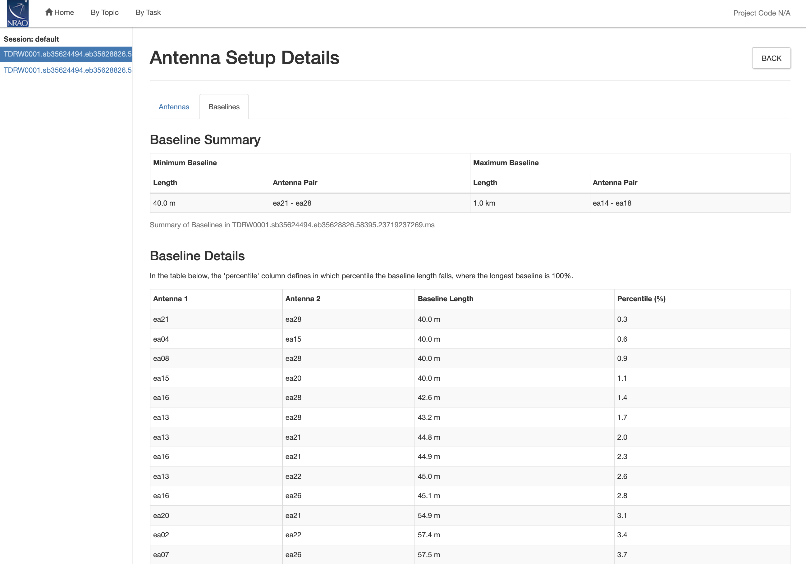
The Antenna Setup (Fig. 4a) page lists the locations of all antennas (antenna pad name and offset from array center) and contains graphical location plots for the array configuration (one linear and one logarithmically scaled for better separation of close antenna labels). A third plot shows a representative uv-coverage. On a second tab, baseline lengths are listed and the 'percentile' column provides a rough indication of how many baselines are shorter than that in each row (Fig. 4b).
Note that antenna IDs are not the same as antenna names. Antennas IDs are assigned when the data are imported to CASA. Thus, antenna ID 1 may or may not be the same as antenna 'ea01'. The Antenna setup page here shows the mapping between IDs and names.
 |
 |
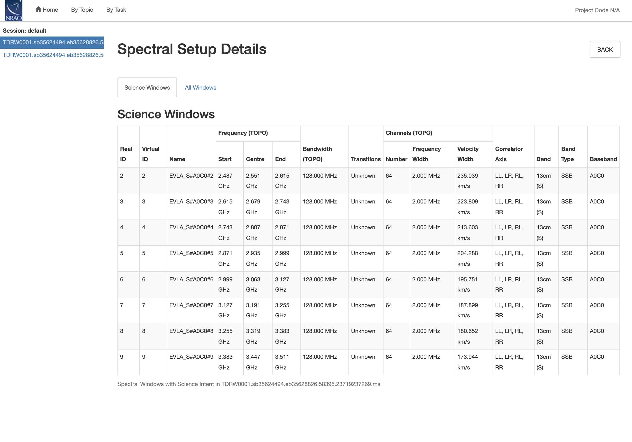
The Spectral Setup page (Fig. 5) contains all spectral window descriptions, including start, center and end frequencies, the bandwidth of each spectral window (spw), as well as the number of spectral channels and their widths in frequency and velocity units. For each spw, the polarization products and the receiver bands are also listed. The real id is the spw id of each SB; the virtual id is a renumbered identifier when multiple SBs are combined (currently only an ALMA option).
Note that Science Windows contain all spws that are used for calibration. Setup and pointing scans are not part of science windows but they are available under All Windows together with their intents.
 |
Clicking the Sky Setup page (Fig. 6) leads to Elevation versus Azimuth and Elevation versus Time plots for the entire observation. The temporal plots are colorized by field id. The page also contains a representative uv-coverage and a solar elevation plot is also shown.
 |
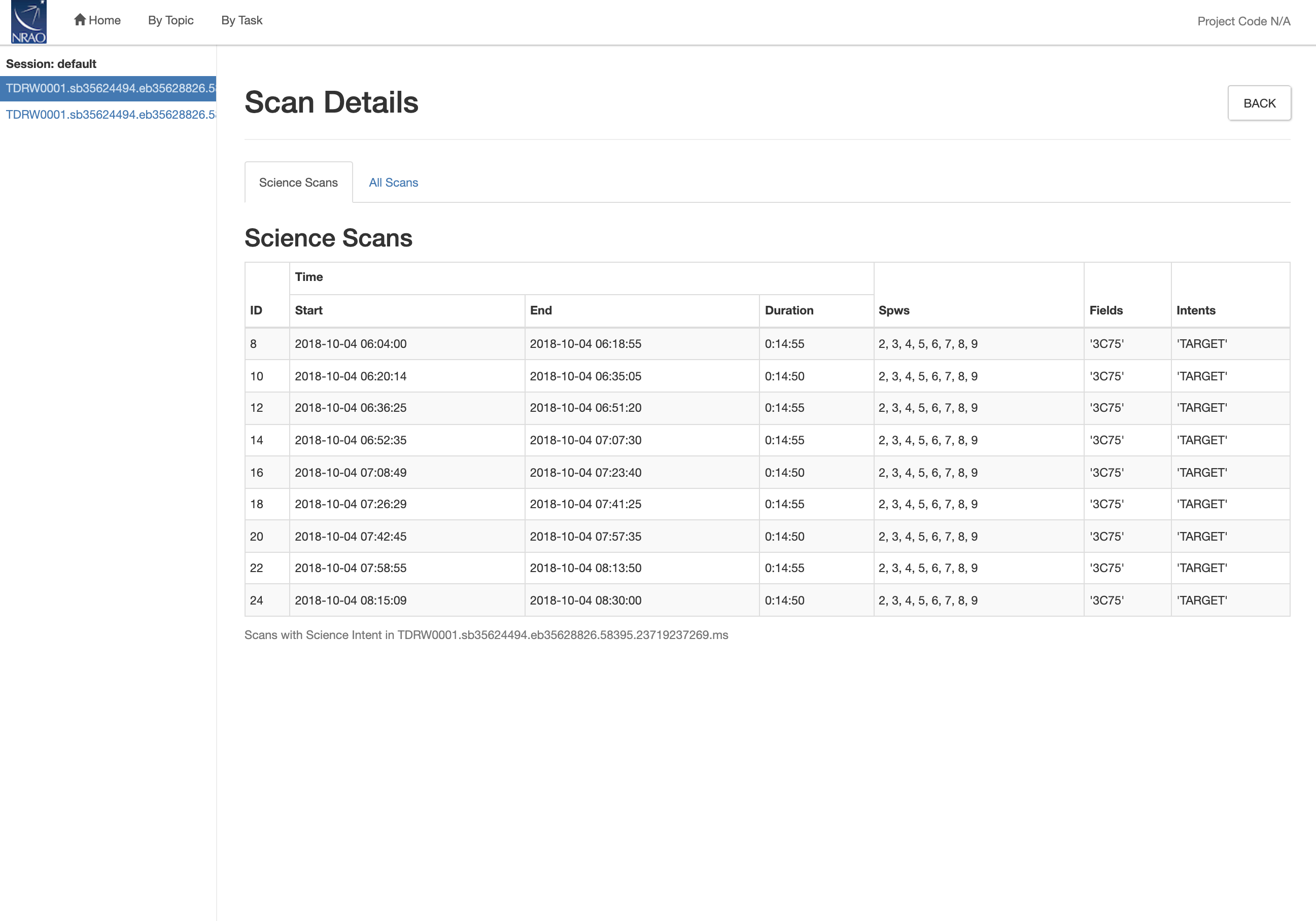
Scans (Fig. 7) provides a listing of all scans, including start and stop time stamps, durations, field names and intents, and the tuning (spw) setup for each. Again Science Scans and All Scans can be inspected in separate tabs.
 |
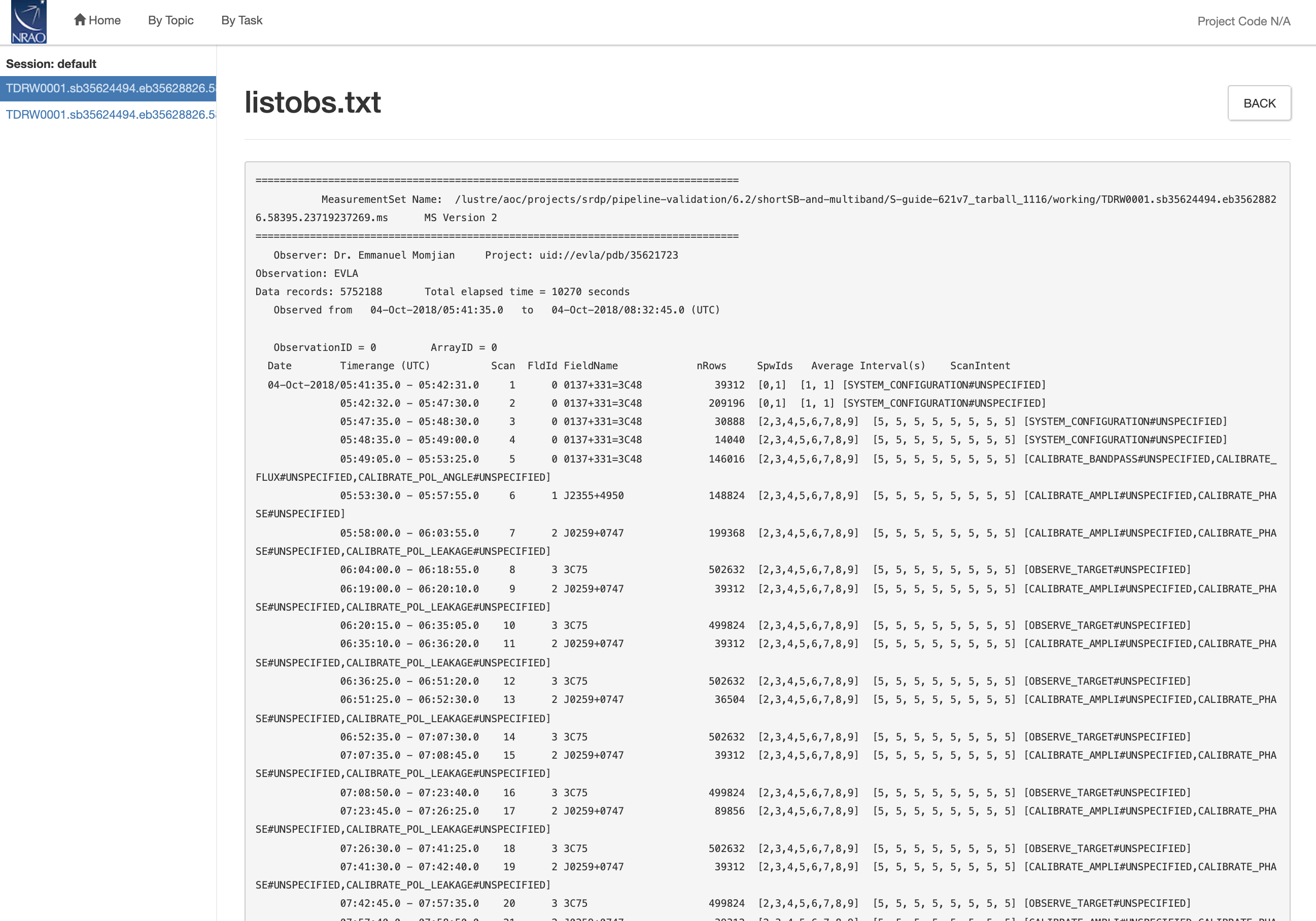
Most of the above information can also be accessed by the 'LISTOBS OUTPUT' button. The link leads to the output of the CASA listobs task, which summarizes the details of the observations (Fig. 8), including the scan characteristics, with observing times, scan ids, field ids and names, associated spectral windows, integration times, and scan intents. Further down, the spectral window characteristics are provided through their ids, channel numbers, channel widths, start and central frequencies. Sources and antenna locations are also part of the listobs output (On some browsers the listobs text is best readable when opened in a new tab without line wrapping).
 |
By Topic Screen
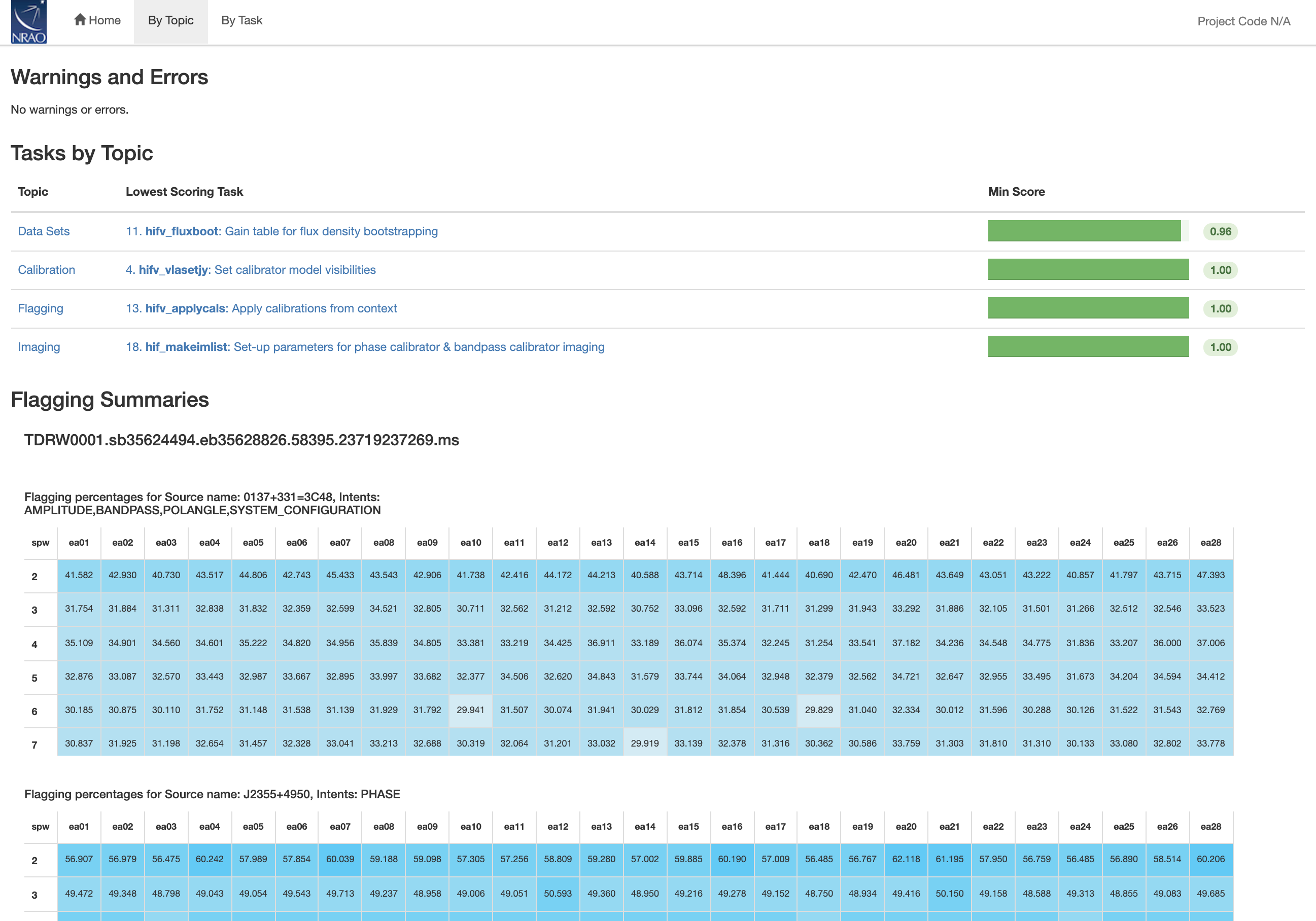
The top-level By Topic link leads to a page that provides basic pipeline summaries such as warnings, the four lowest QA scores (see below), and flagging summaries as functions of field, antenna, and spectral window (spw; Fig. 9). Links are provided to jump directly to the pipeline step that issued the warning or low score.
By Task Screen: Overview of the Pipeline Heuristic Stages
The calibration pipeline is divided into 19 (20 when including the exportdata stage) individual pipeline heuristic stages with heuristic ('hif' or 'hifv' for heuristics interferometric [vla]) tasks listed under the By Task tab (Fig. 10). The imaging pipeline adds another 5 steps for a total of 26 steps in our example (including two archiving exportdata stages). Each stage has an associated score for success. If there are informational messages, warnings, or errors in tasks, they are indicated by '?', '!', and 'x' icons near the task names, respectively. In our example, an informational message and a few warnings are issued, mostly related to flagging.
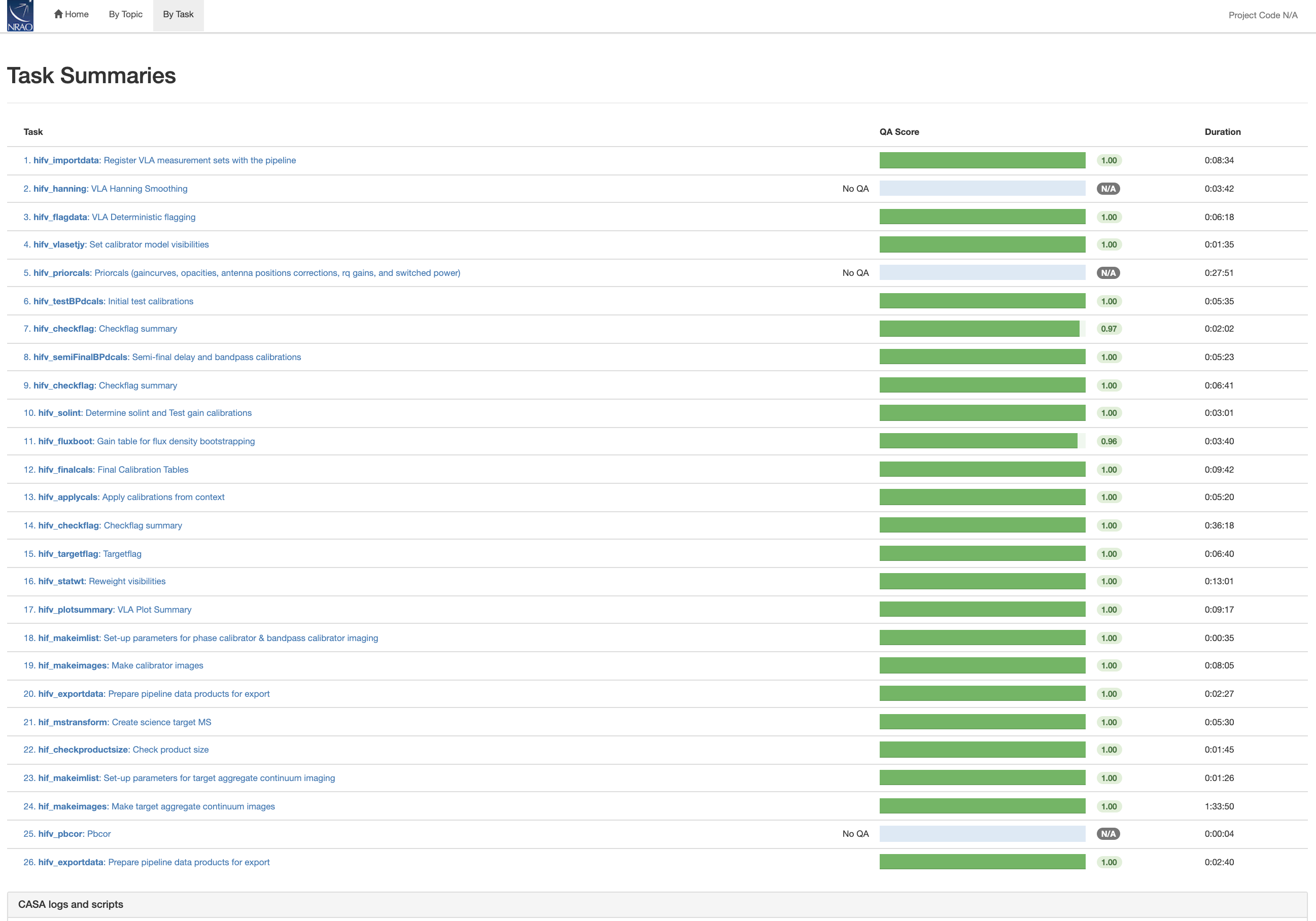
To obtain more details on each stage, click on the individual task name. Task sub-pages contain task results such as plots or derived numbers. Common to all pages is information on the Pipeline QA ('Quality Assurance'), the heuristic task Input Parameters, Task Execution Statistics (benchmarks), and the CASA logs. Those sections provide information on the triggered heuristics, as well as the actual CASA task execution commands and their return logger messages.
The QA scores have the following meaning:
- 0.9-1.0 Standard/Good: green color - the stage appears to have completed successfully
- 0.66-0.90 Below Standard: blue color - the stage has identified some issues, but they are not likely to affect the results substantially. It is still worth a check though.
- 0.33-0.66 Warning: yellow color - there are serious issues identified in this stage. The results should be inspected carefully. Intervention may be needed.
- 0.00-0.33 Error: red color - there are severe problems with the data processing. It may or may not be possible to rescue the data.
The Individual Stages
Before we go through the stages step by step, it is worth mentioning that the lines in the calibration table plots connect data along the x-axis when they have otherwise the exact same properties (i.e. same spw, field, polarization, etc.). When data are flagged the connector will not be plotted, so only consecutive, non-flagged data with the same properties are connected and gaps between data with the same color indicate flagged data.
Stage 1. hifv_importdata: Register VLA measurement sets with the pipeline
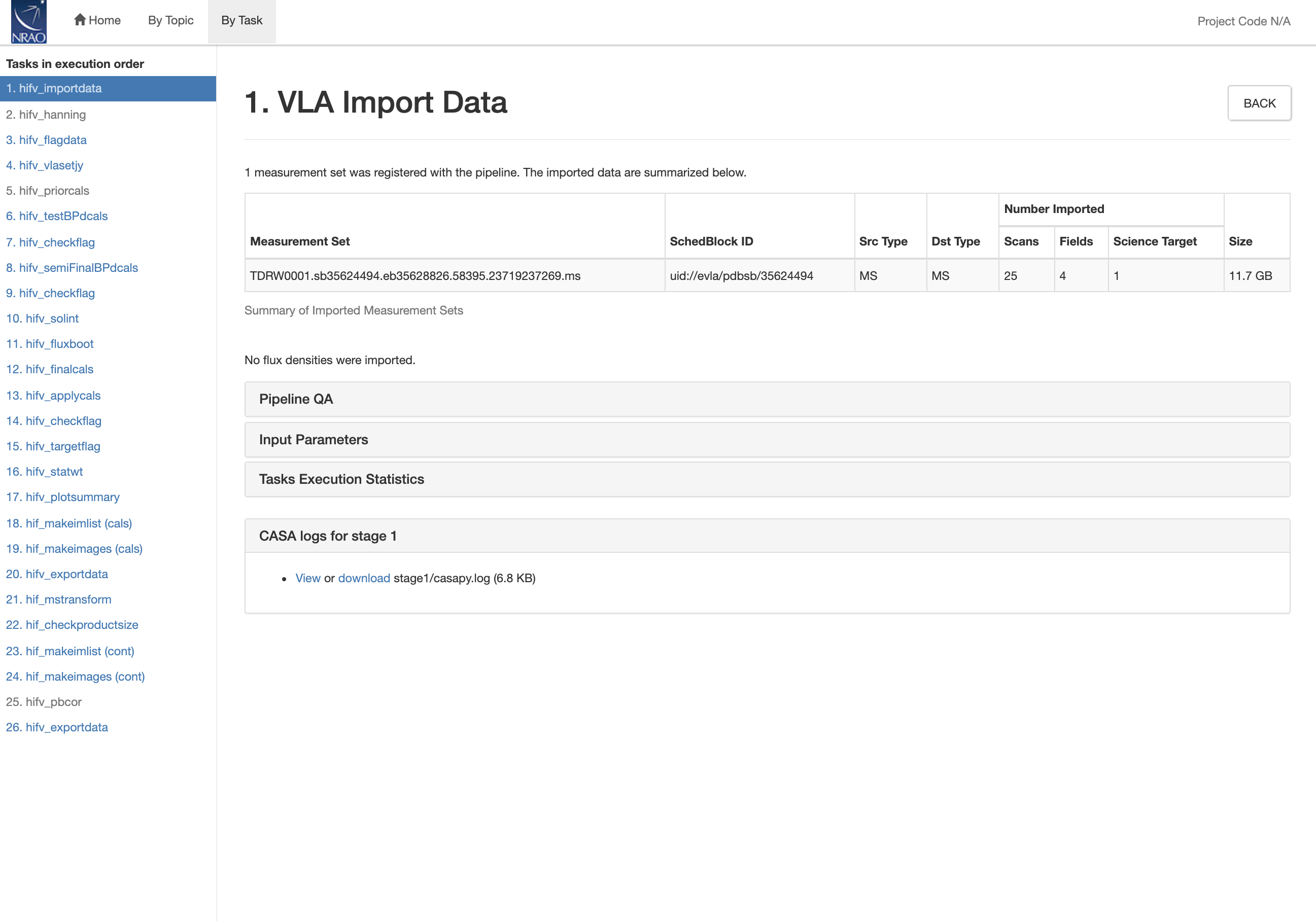
In the first stage, the raw SDM-BDF is imported into the VLA pipeline. An MS is created and basic information on the MS is provided, such as SchedBlock ID, the number of scans and fields, science targets, and the size of the MS. The MS is also checked for suitable scan intents and a summary of the initial flags is calculated (check the "CASA logs" attached to the bottom of the page).
 |
CHECK for: any errors in the import stage. Warnings will also be issued for missing, necessary scan intents or if the data had previously been processed. This is usually encountered when the pipeline is run on an MS rather than an SDM.
QA: If the INTENT PHASE or FLUX are missing, the score will be set to 0. An existing processing history will set it to 0.5.
Stage 2. hifv_hanning: VLA Hanning Smoothing
This stage Hanning-smooths the MS. This procedure reduces the Gibbs phenomenon (ringing) when extremely bright and narrow spectral features are present and spill over into adjacent spectral channels. Gibbs ringing is typically caused by strong RFI or a strong maser line. As part of the process, Hanning smoothing will reduce the spectral resolution by a factor of 2 while maintaining the same number of channels. (Note: this means that data in adjacent channels will no longer be independent.) The first and last edge channel will be flagged. Hanning smoothing is turned off when any spectral window (spw) was frequency-averaged inside the WIDAR correlator. For such data, Hanning smoothing cannot correct for the Gibbs phenomenon anymore and would only add additional smearing.
CHECK for: nothing except for completion of the task. FOR SPECTRAL LINE DATA: you may decide not to run this stage since spectral lines will be smoothed to a degraded spectral resolution.
QA: N/A
Stage 3. hifv_flagdata: VLA Deterministic flagging
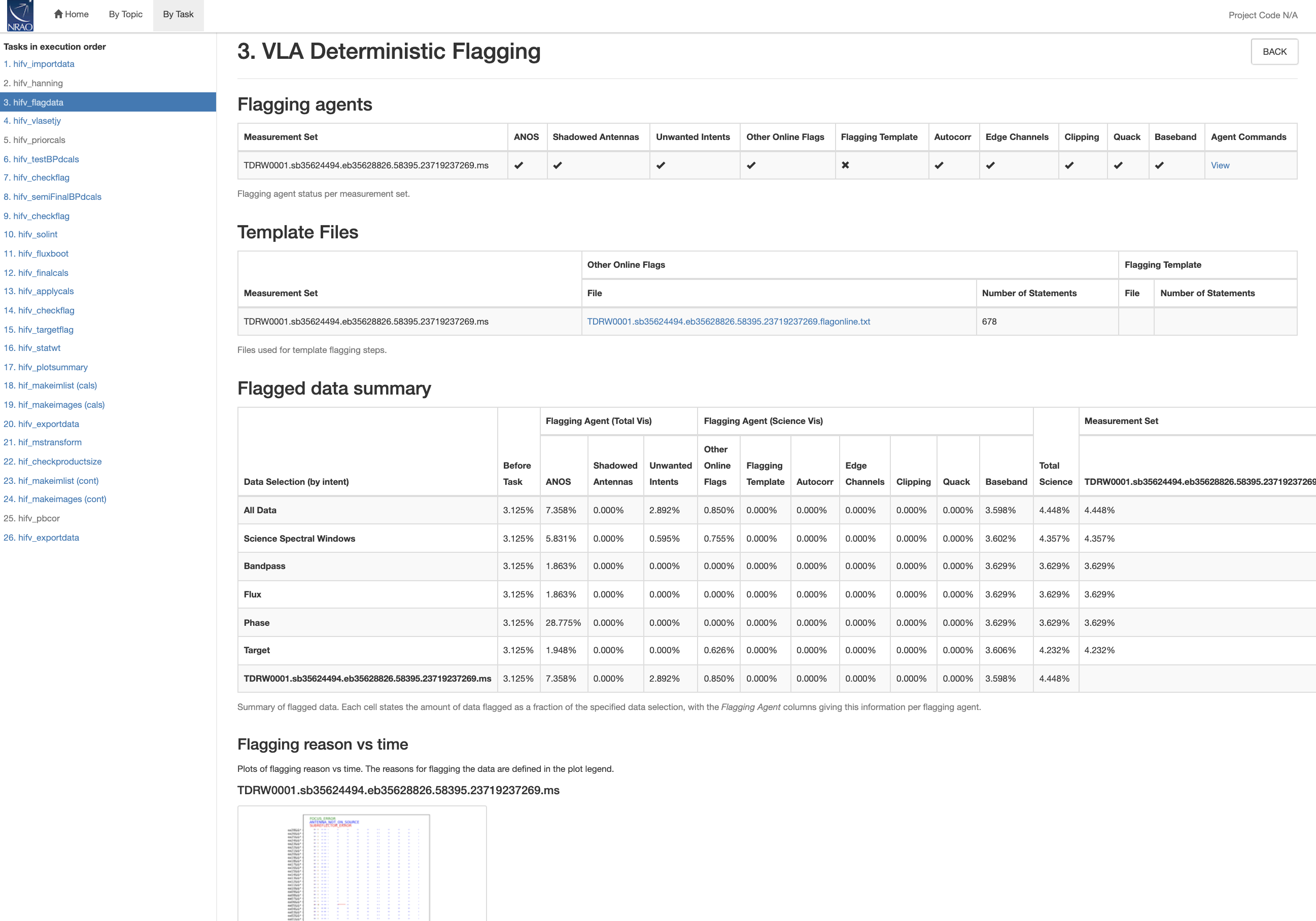
This stage applies flags that were generated by the VLA online system during the observations. The flags include antennas not on source (ANOS), shadowed antennas, scans with intents that are of no use for the pipeline (such as pointing and setup scans), autocorrelations, the first and last 5% edge channels of each spectral window (with a minimum of 1 channel), clipping absolute zero values that the correlator occasionally produces, quacking (i.e. flagging start or end integrations of scans; the pipeline will flag the first integration after a field change), and flagging the end 20MHz of the top and bottom spw of each baseband (when the baseband is <1GHz, the baseband flagging will be disabled). "Agent Commands" is the actual list of flagging commands that is sent to the CASA task flagdata. The flags are reported as a fraction of the total data for the full dataset as well as broken up into the individual calibrator scans and target data (according to their intents). A plot is provided that displays the online antenna flags as a function of time.
A flagging template can also be provided to the pipeline which applies known flags to the data (see The VLA Pipeline Webpage). These templates are created by a user before starting the pipeline. They are also prepared by NRAO staff for Science Ready Data products when needed.
In our example (Fig. 12), the target sources start with 3.125% flagged data that are due to Hanning smoothing, which flags the first and last channel of each spw (2 out of 64 channels in our case). The deterministic flagging stage adds various ANOS, baseband, and other flags (e.g. subreflector rotation, like the error in ea05 as plotted in the graph) for a total 4.4%. No flagging template was applied.
 |
CHECK for: the percentage of the flags. If a very large portion (or even all) of the visibilities of the calibrators are flagged, try to find out the reason. Also have a quick look at the graph of the online flags to understand whether the system behaved normally or if there was an unusually high failure of some kind.
QA: Determined by the percentage of incremental flagging where 0 < score < 1 is the score range for 60% < fraction flagged data < 5%.
Stage 4. hifv_vlasetjy: Set calibrator model visibilities
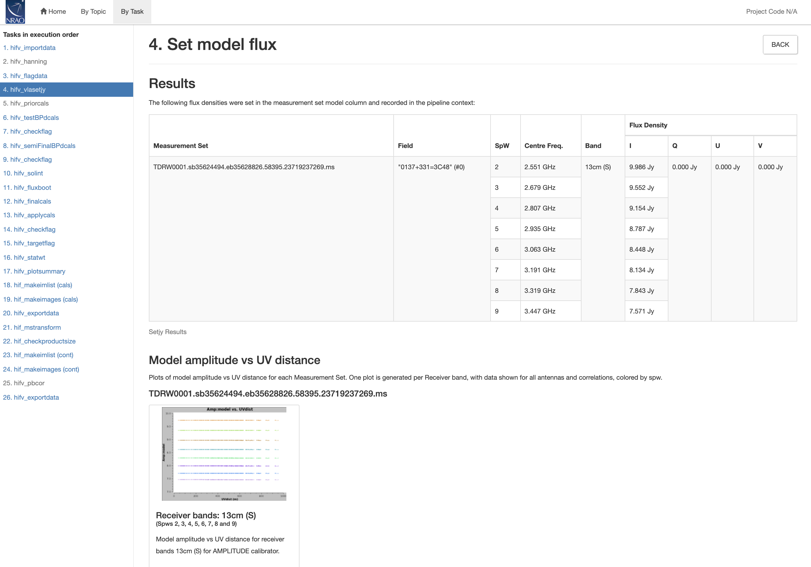
Stage number 4 calculates and sets the calibrator spectral and spatial model for the standard VLA flux density calibrators (3C48, 3C138, 3C147, or 3C286 with a CALIBRATE_FLUX scan intent). The task page (Fig. 13) lists the calculated flux densities for each spectral window (spw). It also contains plots of the amplitude versus uv-distance for the models per spw that are calculated and used to specify the flux density calibrator characteristics. Our example uses 3C48, and for this array configuration and band the source appears largely as a point source given the flat uv-distance amplitudes. The spectral index, however is visible in the colored spws that are at different flux density levels.
If the scan intent CALIBRATE_FLUX is absent the pipeline will not run. If the calibrator is not a standard VLA flux density calibrator, the absolute flux density scale calibration will be on an arbitrary level.
 |
CHECK for: any unexpected flux densities or model shapes.
QA: If the flux calibrator is not one of the VLA flux standards (3C48, 3C138, 3C147, 3C286), the score will be 0.5.
Stage 5. hifv_priorcals: Priorcals (gaincurves, opacities, antenna positions corrections and rq gains)
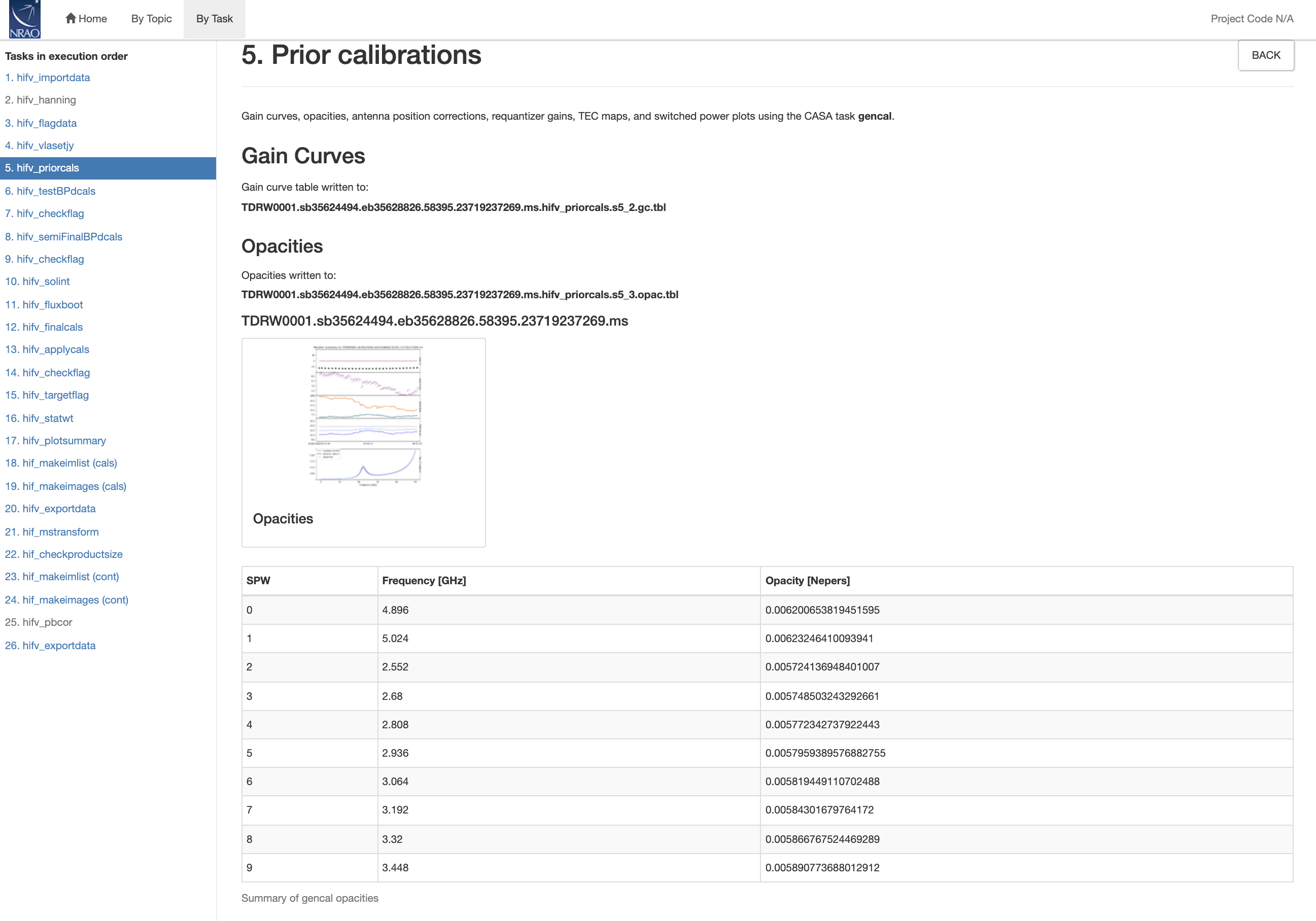
Next, the prior calibration tables are being derived. They include gain-elevation dependencies, atmospheric opacity corrections, antenna offset corrections, and requantizer (rq) gains. They are independent of the calibrator observations themselves and can be derived from ancillary data such as antenna offset tables, weather data, and antenna elevation. Switched power measurements are provided but currently not used in the pipeline. They can be manually inspected, e.g. for gain compression in the presence of strong RFI.
Opacities are calculated per spw and plotted together with additional information on the weather conditions during the observation (Fig. 14a). For S-band they are very low, as expected for frequencies that are largely unaffected by water vapor.
 |
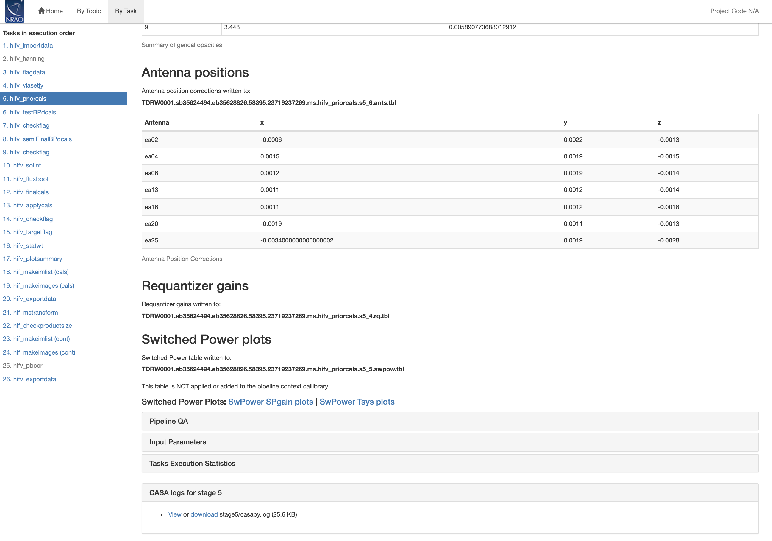 |
The antenna positions are usually updated within a few days after an antenna was repositioned during the cycle (Fig. 14b). For our case, however, 7 antennas have updated positional corrections (on the order of a few millimeters) that will be applied during calibration.
CHECK for: extreme or unrealistic opacities. Also check that the antenna offsets are within are reasonable range (reasonable values are usually less than +/- 0.0200 meters). There should only be updates for a few antennas.
QA: N/A; but a warning will be issued when more than 50% of antennas need position corrections, or when the weather station data are absent for observations at K-band frequencies and above.
Stage 6. hifv_testBPdcals: Initial test calibrations
Now it is time to determine the delays and the bandpass solutions (gain and phase) for the first time. Applying the initial solution will make it easier to identify RFI that needs to be flagged. There will be a couple of similar iterations for the calibration tables in the following pipeline stages to eventually obtain the final set of calibration tables.
The plot on the main page (Fig. 15) shows the bandpass calibrator with the initial bandpass solutions applied. There are links to other plots showing delay, gain amplitude, gain phase, bandpass amplitude, and bandpass phase solutions for each antenna. Note that the pipeline will typically switch reference antennas, and therefore phase solutions of reference antennas may not be perfectly zero and may show some steps. When delays are more than +/-10ns it will be worth examining the data more closely. Some additional flagging may be needed.
 |
The gain amplitude and phase solutions are derived per integration and they are used to correct for decorrelation before any spectral bandpass solutions are calculated (note that later stages do not show this plot anymore). The latter are determined over a full solution interval, usually for all bandpass scans together. Bandpasses should be smooth although they can vary substantially over wide frequency bands. The bandpass (BP) phase solutions are derived after systematic slopes were accounted for by the delay solutions.
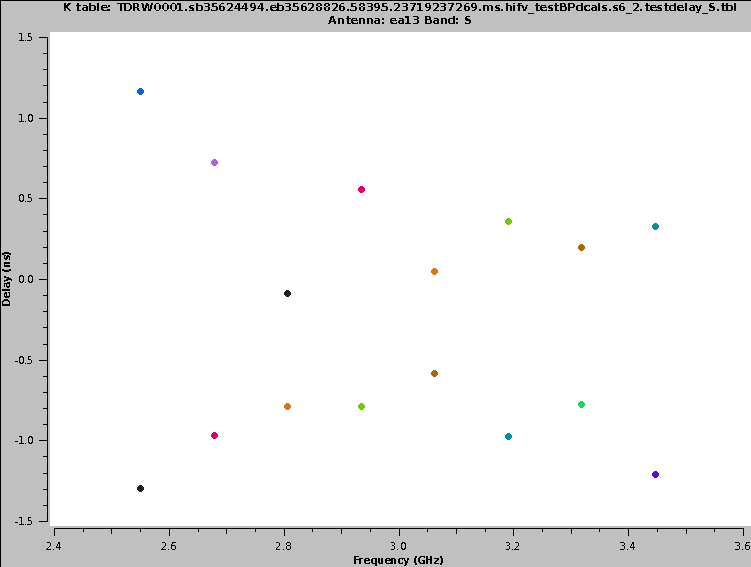
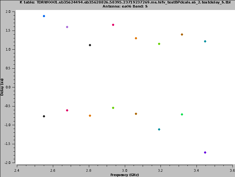
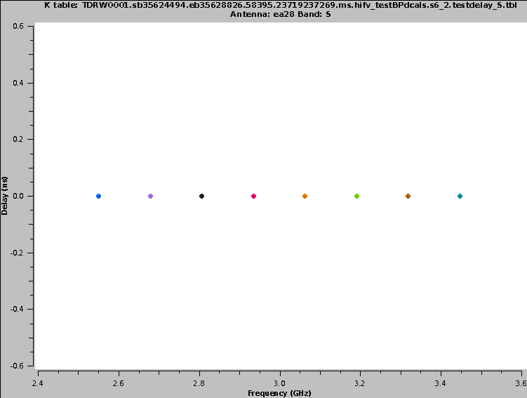
Example delays are shown in Fig. 16a-c: The delays for ea13 vary but are within a narrow range of only a few ns (and small offsets between spws)(Fig. 16a). These are good solutions. The delays for ea13 and ea06 are fine given that they are only a few ns. Ea06 furthermore shows a systematic offset of the delays between the polarizations (Fig. 16b). This is nothing to worry about. Delays for ea28 are all zero (Fig. 16c). This is expected as ea28 is the reference antenna. Very large delays of hundreds of ns, very different delays between spws, random scatter or systematic problems (antenna, correlator, RFI, etc), should be flagged.
 |
 |
 |
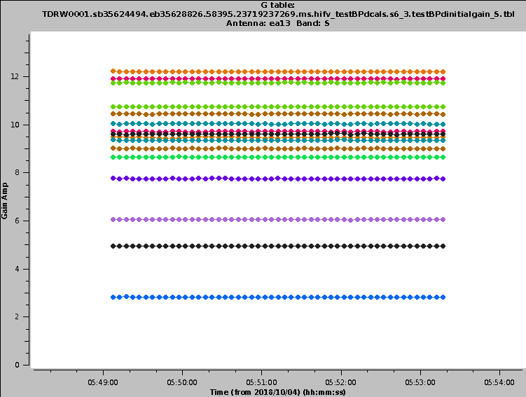
The gain as a function of time for ea13 is shown in Fig. 17. It is flat and well behaved per spw. Offsets between the colored spws will be taken out as part of the calibration.
 |
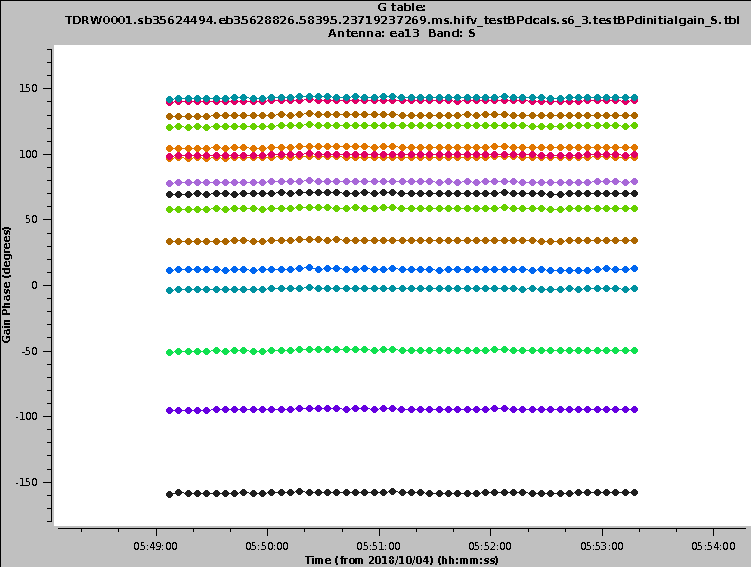
Since the gain amp/phase steps per integration are only performed to reduce decorrelation, the phase plots are the most important diagnostics in this context. In Fig. 18 we show the solutions for ea13. They are flat and well behaved again, little decorrelation is visible that this table would correct for.
 |
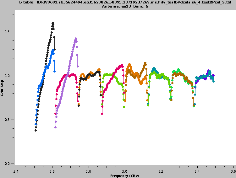
Now let's have a look at the bandpasses themselves (Fig. 19). Antenna ea13 is again a good representative for all antennas. The colored spws are clearly distinguishable (2 polarizations plotted on top of each other). Edge channels show lower gain, in particular at the edge of the baseband, below ~2.6GHz.
 |
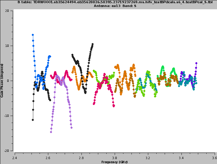
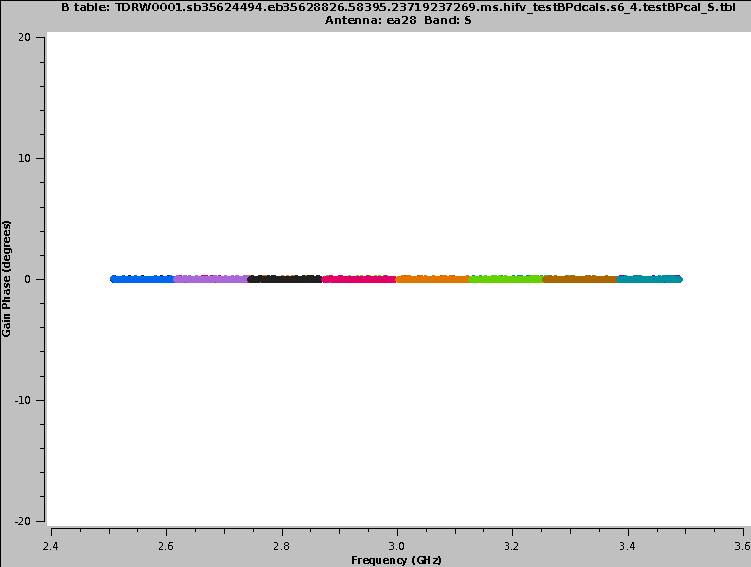
The bandpass (BP) phases as a function of frequency/channel are shown in Fig. 20a-b. Spw edges have large phase changes, but they are still only a few degrees (Fig. 20a). Ea28 phases are zero, as expected for the reference antenna (Fig. 20b).
 |
 |
Flagging bad deformatter data
Included in this stage is the detection and removal of data transmission problems (aka 'bad deformatter' issue). A description of the effect is provided on the Pipeline: Frequent VLA problems page.
CHECK for: strong RFI and whether it was eliminated in later flagging stages or not (especially via a comparison with the output plots of stage 12). Also check for jumps in phase and/or amplitude away from spectral window edges. If there are phase jumps for all but the reference antenna, maybe a different choice for the reference antenna should be considered. Also watch out for extreme delays of tens of ns and for very noisy data.
QA: checks are performed for the presence of delay and bandpass solutions for all science spws and antennas. The fraction of failed bandpass solutions changes the score to 0 < score < 1 for 60% < failed solutions < 5%. The score is furthermore reduced by 0.1 for every antenna where delays exceed >200ns.
Stage 7. hifv_checkflag: Flag possible RFI on BP calibrator using rflag
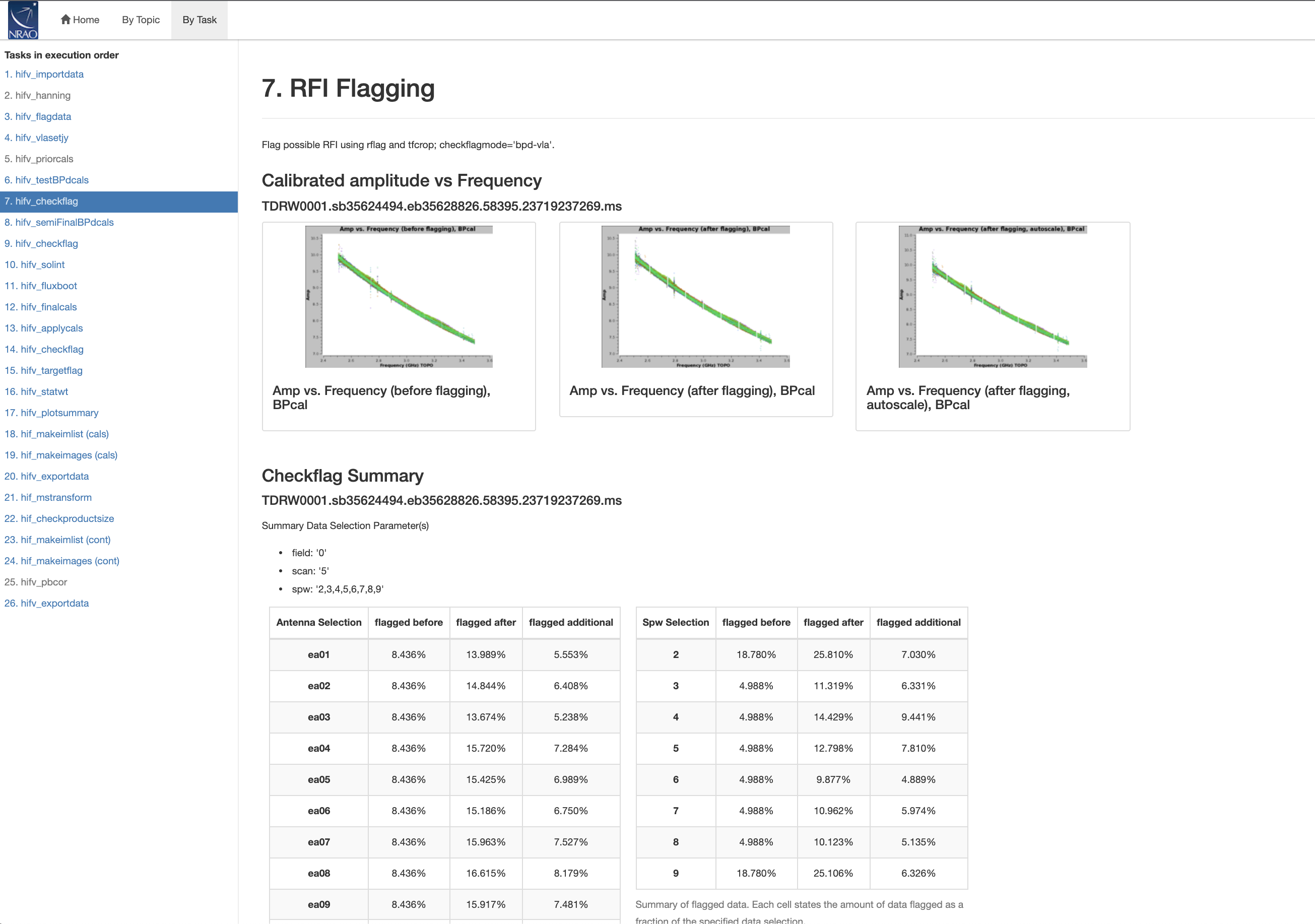
Rflag as part of CASA's flagdata is a threshold-based automatic flagging algorithm in CASA. Tfcrop is a 2D (frequency/time) flagging algorithm that works on uncalibrated data. A combination of the two algorithms is run on the bandpass calibrator to remove relatively bright RFI and to obtain improved bandpass calibrations tables later on. The plots in Fig. 21 show the data before and after flagging. Note that sometimes the plots after flagging look worse, which is typically due to different averaging of the data.
 |
CHECK for: RFI removal in the diagnostic plots and subsequent processing stages. Check if there are specific antenna/spw combinations that have high flagging percentages, and which may be better flagged entirely.
QA: determined by the percentage of incremental flagging where 0 < score < 1 is the score range for 60% < fraction flagged data < 5%.
Stage 8. hifv_semiFinalBPdcals: Semi-final delay and bandpass calibrations
Now that some RFI was flagged, stage 6 is repeated here at stage 8, which results in better bandpass and delay solutions. The warning is the same as in stage 6.
CHECK for: strong RFI and whether it was eliminated in later flagging stages or not (especially via a comparison with the output plots of stage 12). Also check for jumps in phase and/or amplitude away from spectral window edges. If there are phase jumps for all but the reference antenna, maybe a different choice for the reference antenna should be considered. Also watch out for extreme delays of tens of ns and for very noisy data.
QA: checks are performed for the presence of delay and bandpass solutions for all science spws and antennas. The fraction of failed bandpass solutions changes the score to 0 < score < 1 for 60% < failed solutions < 5%. The score is furthermore reduced by 0.1 for every antenna where delays exceed >200ns.
Stage 9. hifv_checkflag: Flag possible RFI on all calibrators using rflag
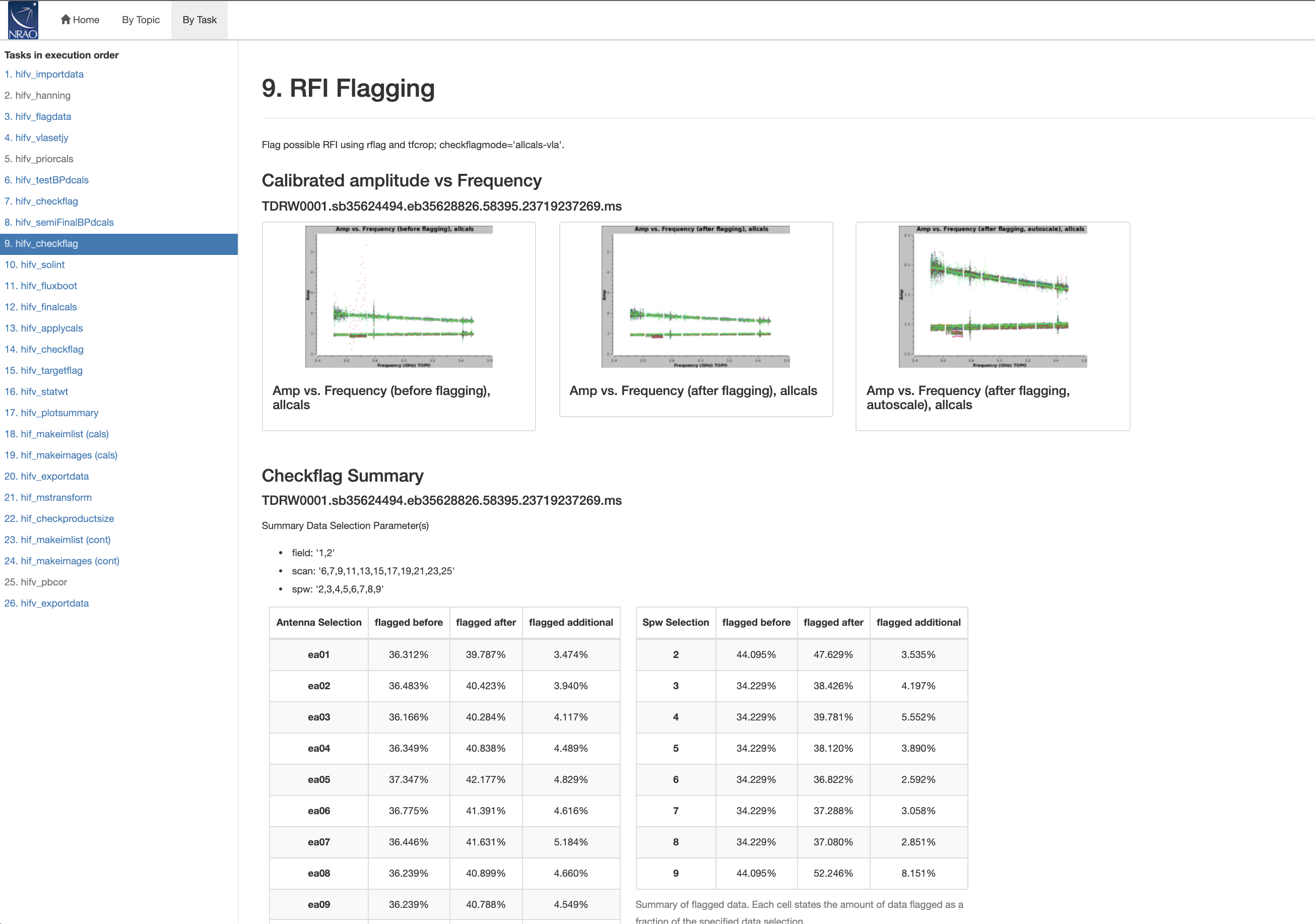
Once more, tfcrop and rflag are executed, this time on all calibrator scans (Fig. 22). For the bandpass, after the bright RFI has been removed in stage 7 and a new bandpass solution has been applied in stage 8, a new flagging threshold will account for weaker RFI, which will be removed here in stage 9. The RFI is somewhat reduced but not fully removed. The complex gain calibrator (all calibrators are in common plots) shows an amplitude drop in a small frequency range around 2.7GHz, likely one spw. The calibration will take that into account.
 |
CHECK for: RFI removal in the diagnostic plots and subsequent processing stages. Check if there are specific antenna/spw combinations that have high flagging percentages, and which may be better flagged entirely.
QA: determined by the percentage of incremental flagging where 0 < score < 1 is the score range for 60% < fraction flagged data < 5%.
Stage 10. hifv_solint: Determine solint and Test gain calibrations
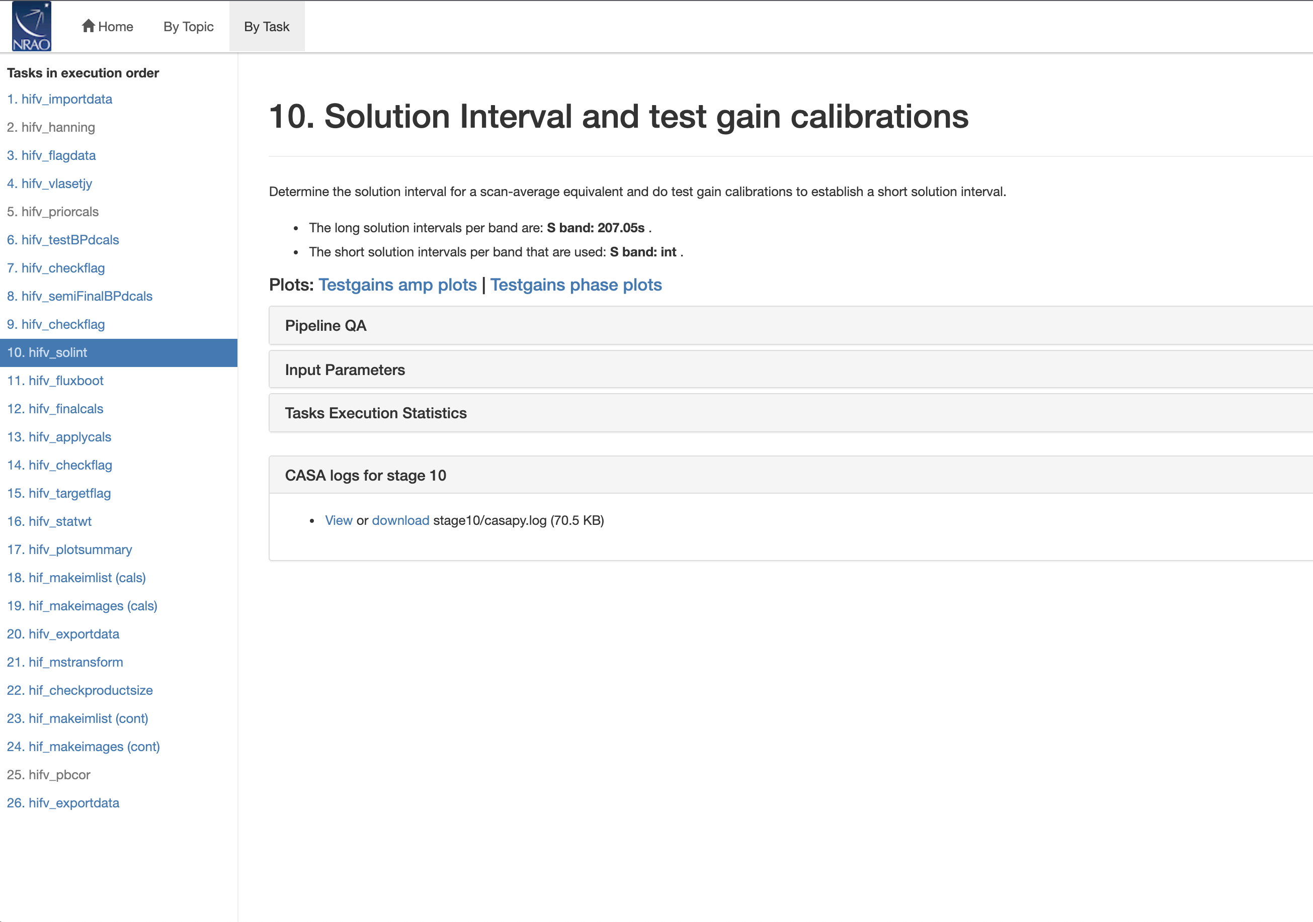
For the final calibration, the pipeline determines the shortest and longest applicable solution intervals (solint). Typically the short solint is a visibility integration (dump) time interval; the longest of those are used when they differ during the observations. The long solint is derived from the length of the longest gain calibration scan.
In our case (Fig. 23) the longest solution interval, capturing the length of gain calibrator scans after flagging, is 207s. The short solution interval is 'int', which corresponds to one integration length, or 5s (cf. the overview page).
 |
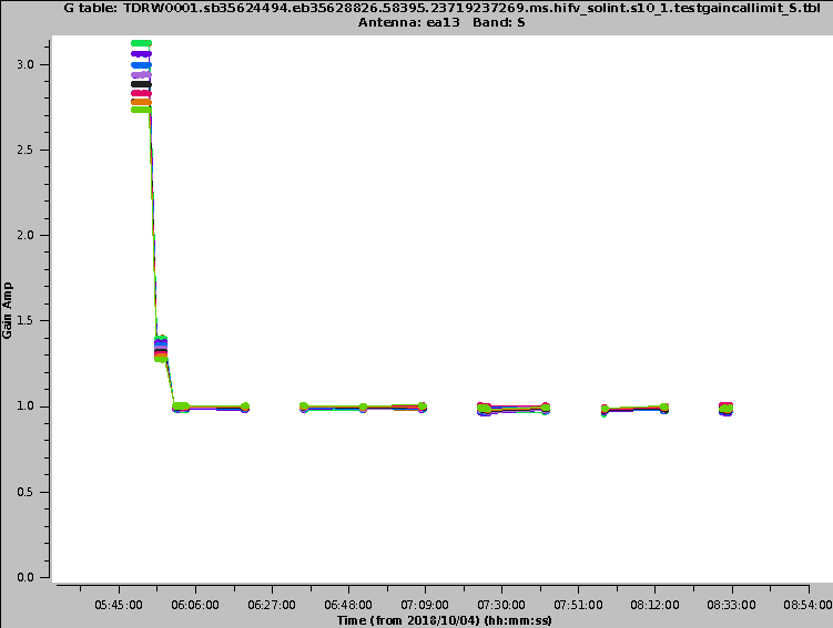
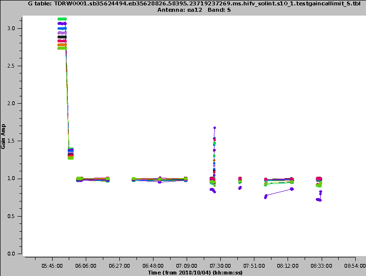
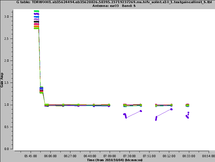
Initial temporal gain and phase solutions are calculated for each antenna, spectral window, and polarization using these time intervals. In Fig. 24a-d we show some examples for the gains. At this stage, the solutions are already quite good. The variations are very small, as can be seen for the representative antenna ea13 (the amplitude offsets between the scans are the different calibrator sources that are observed) (Fig. 24a). Antenna ea12, however, has some anomaly at around 7:28UT that the pipeline may try to flag (Fig. 24b). It should be flagged by hand, if the pipeline will not address it for the final calibration tables (stage 12). Also ea03 shows lower gain solutions in the second half of the run. That may need to be flagged, but could also reflect a true lower gain of that antenna in some spw/polarization (Fig. 24c).
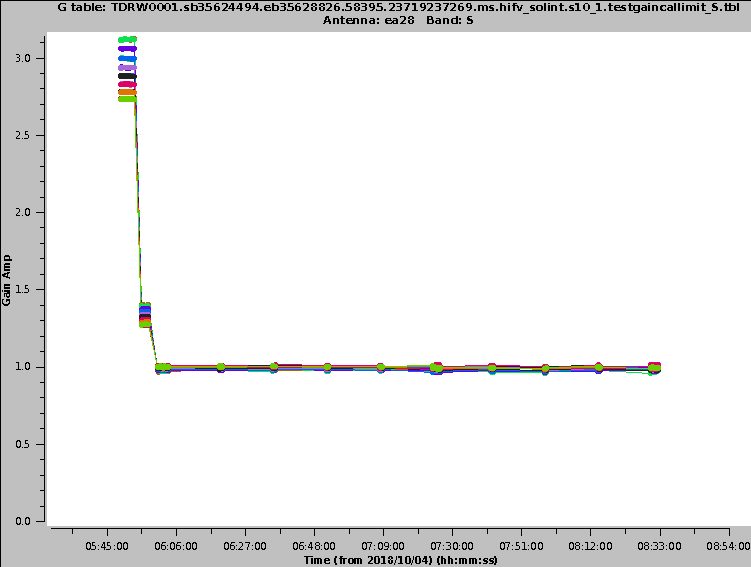
Given the plotting algorithm, lines only connect the exact same setup (antenna spw, pol, etc). Flagged data will not be connected. The plots therefore sometimes look different in their visual appearance with connected lines sometimes even criss-crossing. E.g. ea28 has little flagging and most connectors are present whereas for other antennas the connectors are broken at flag boundaries (Fig. 24d).
 |
 |
 |
 |
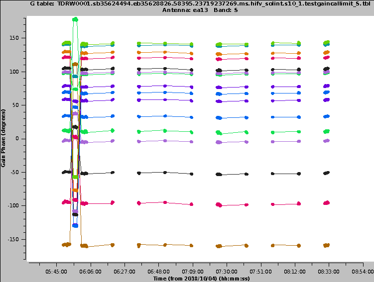
Phase solutions are provided in Fig. 25a-d for antennas ea13, ea28, and ea18. Ea13 shows reasonably flat phases with little variations, except for phase jumps between different calibrators (Fig. 25a). The almost vertical lines seen for ea18 are irrelevant as they are connectors for -180 to 180 degree phase wraps (Fig. 25b). Ea28 is again the reference antenna with zero phases (Fig. 25c). For the calibrator around 5:55 UT, J2355+4950, however, the phases for ea28 spread out, indicating that a different antenna was the reference at that point. Indeed, ea19 shows zero phases for that scan and was used as the reference antenna at that time (Fig. 25d).
 |
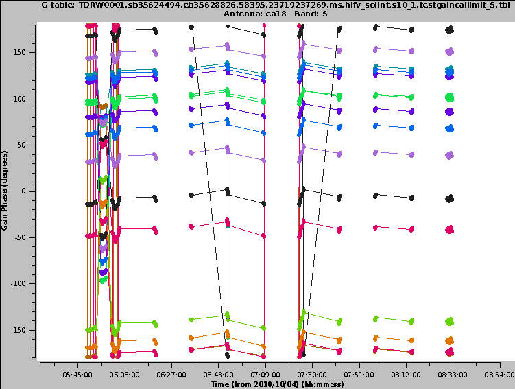 |
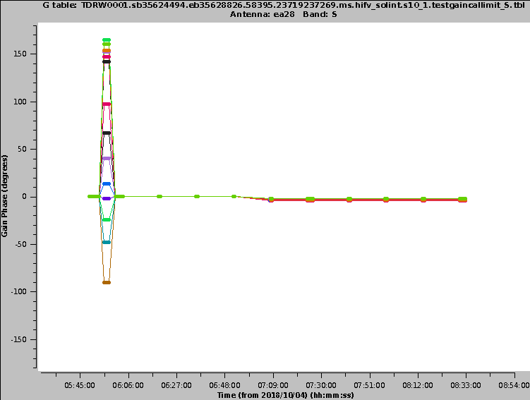 |
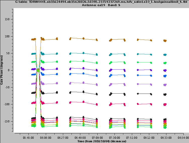 |
CHECK for: consistency with the data. The shortest solution interval should be close to the (longest) visibility integration time and the longest gain calibration scan. Gains should be smooth with little variations in time (where larger gain variations are more likely to occur for higher frequencies), phases should not show any jumps and should be relatively smooth in time (where larger phase variations are likely to occur for higher frequencies and longer baselines).
QA: N/A; but a warning will be issued when the long and short solint values are the same +/- one integration.
Stage 11. hifv_fluxboot: Gain table for flux density bootstrapping
Now, the flux densities are bootstrapped from the flux density calibrator to all other calibrators, including the complex gain (amplitude and phase) calibrator. To do so, polynominal functions are fitted for the secondary calibrators and the absolute flux densities are determined for each spw. They are then inserted in the MODEL column via setjy and reported for each spectral window.
For our example, the pipeline derives frequency-dependent flux densities between 0.94 and 0.99 Jy for 'J0259+0747' and 1.94 to 1.62 Jy for 'J2355+4950', the two calibrators that are observed with a PHASE intent. This is reflected in the polynomial fit results, where one source has a positive and the other a negative spectral index, also shown by the fits in the fourth panel in Fig. 26. The third panel shows the (very small) residual errors of the fits. A gaintable ('fluxgaincal.g') is generated based on these numbers and shown in the first plot, based on the source model that is shown in the second plot. If the plots show RFI or badly calibrated data, it is possible to edit the 'fluxgaincal.g' file using e.g. plotms. The VLA pipeline webpage has instructions on how to insert an edited table into the calibration run.
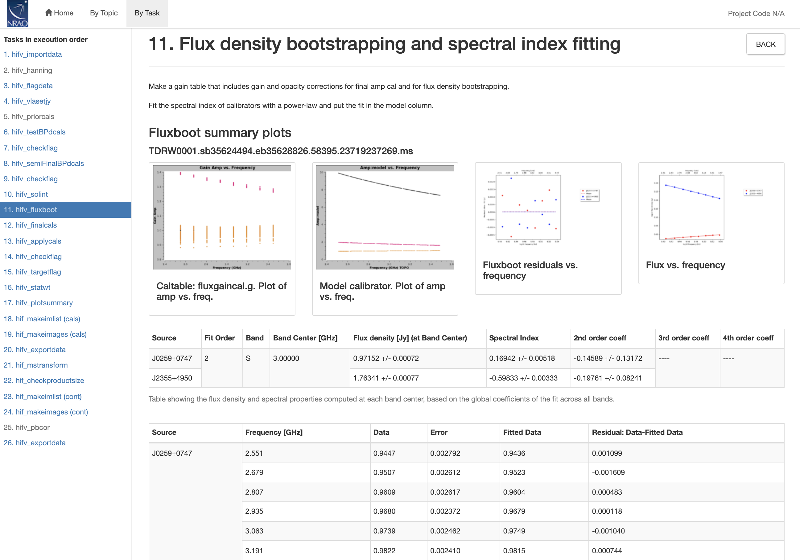 |
CHECK for: that the flux density values are close to the known values for the calibrator. Check the VLA calibrator manual at https://science.nrao.edu/facilities/vla/observing/callist for consistency. Since most calibrator sources are time variable AGN, some differences to the VLA catalog are expected. In particular, at higher frequencies they could be different by up to tens of percent.
QA: based on the S/N and maximum residual of the fit. A fraction of 0.01 is deducted from a max score of 1.0 for each residual that is more than 1 sigma away from the mean. This value is calculated per source and normalized over all sources.
Stage 12. hifv_finalcals: Final Calibration Tables
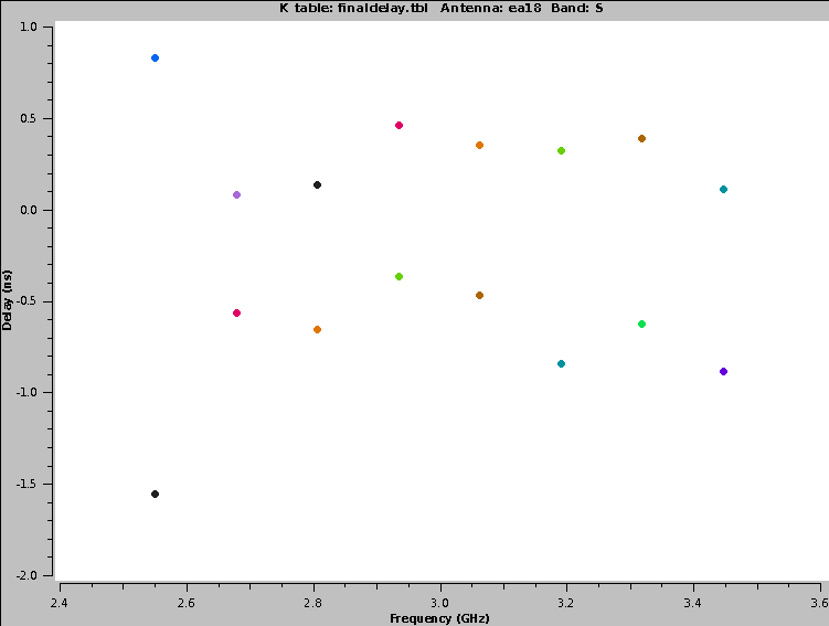
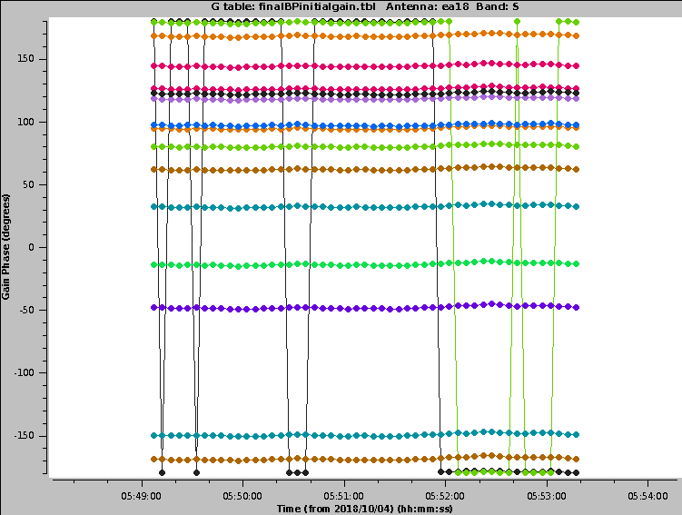
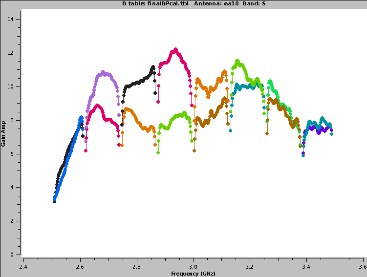
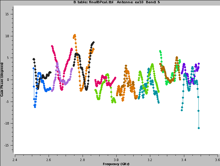
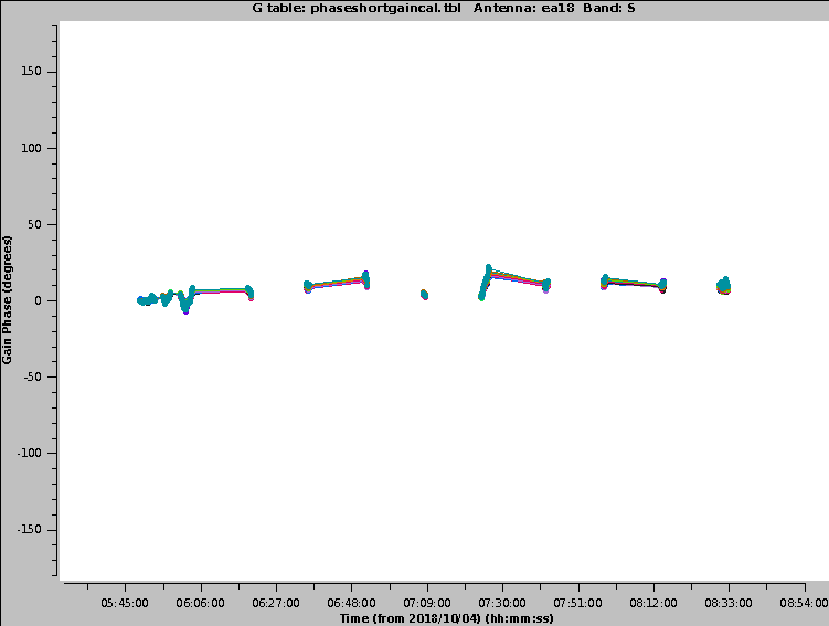
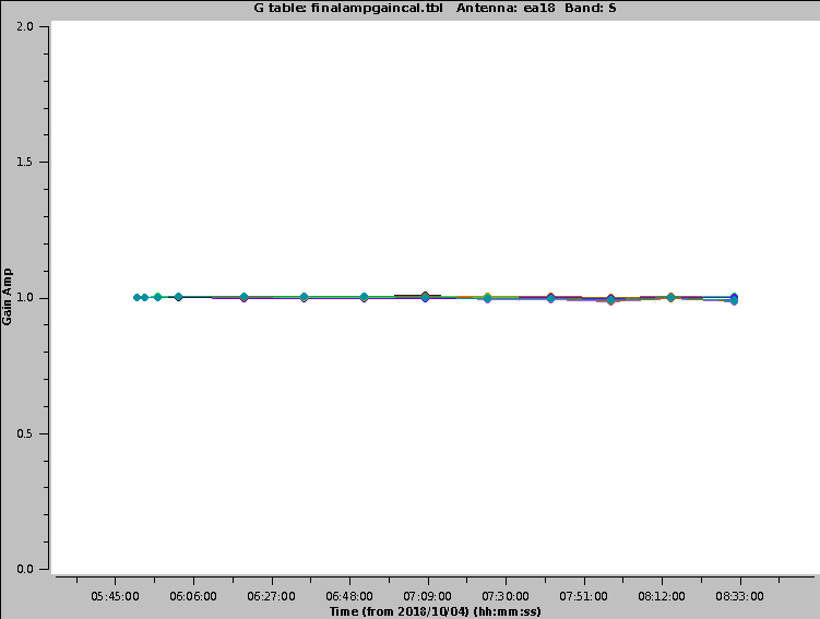
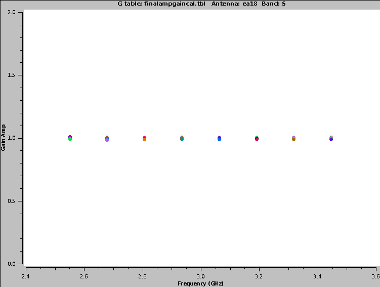
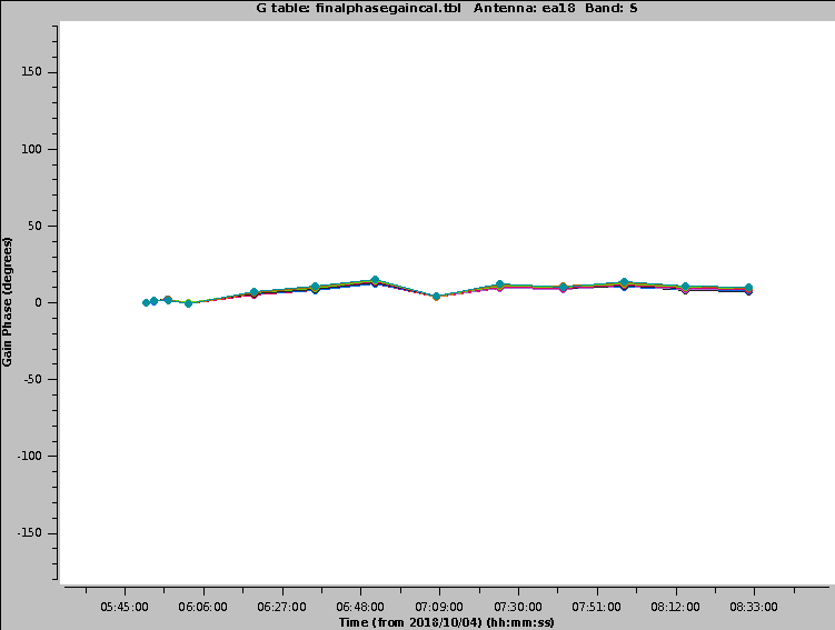
The final calibration tables are now derived. Those are the most important ones given that they are actually applied to the data in stage 13. The tables, which contain antenna based solutions, are: Final delay, bandpass (BP) initial gain phase, BP Amp solution, BP Phase solution, Phase (short) gain solution, Final amp time cal, Final amp freq cal, and Final phase gain cal. In Fig. 27a-h, we show an example of each of these for ea18. For this antenna all of the data look good. Bandpasses are smooth (although steep at the lower frequency end), phase solutions are within a few degree and gains (temporal and spectral) are close to unity with little deviation. The short phase solution is also pretty flat, indicating that decorrelation is very low.
 |
 |
 |
 |
 |
 |
 |
 |
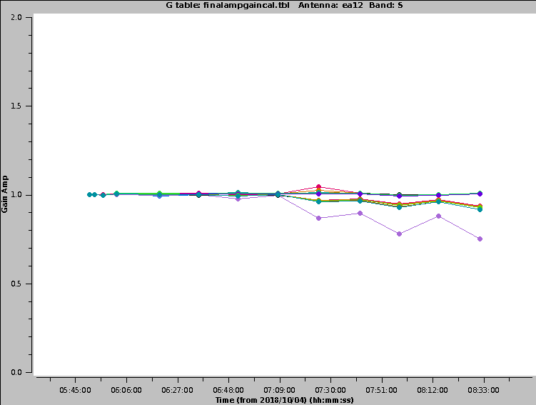
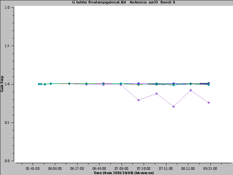
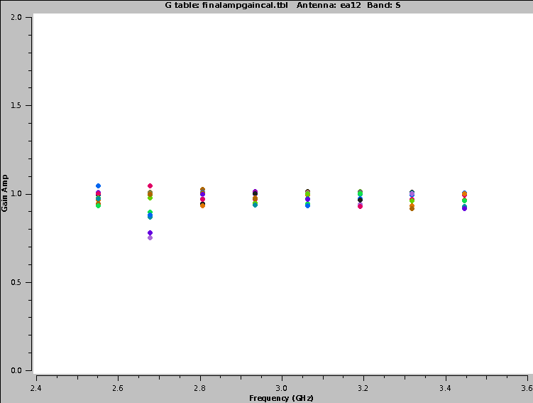
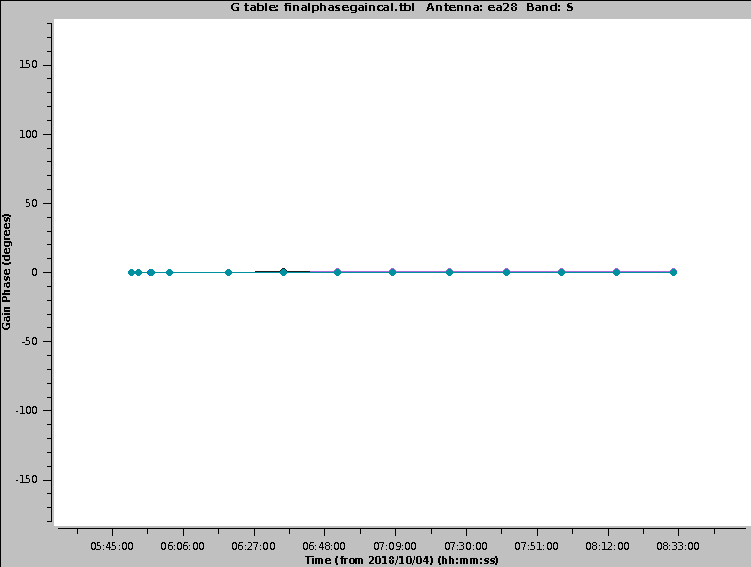
Some antennas, however, show some problems (Fig. 28a-d). The gains for ea12 and ea03 start deviating from their ideal value for a few spws at about half of the observing run (Fig. 28a-b). This could be flagged. Also one spw for ea12 shows a spread around 2.67 GHz (Fig. 28c). That could be flagged, too. Ea28 is only displayed to show that this one is the phase reference (Fig. 28d).
 |
 |
 |
 |
CHECK for: strong RFI as well as jumps in phase and/or amplitude away from spectral window edges. If there are phase jumps for all but the reference antenna, maybe a different choice for the reference antenna should be considered. Also watch out for extreme delays of tens of ns and for very noisy data.

Note that carefully checking calibrator tables in this stage is of particular importance as they are the final tables that are applied to the target source. Phase (and gain) calibration solutions should be inspected in their temporal variations to be smooth and consistent for each calibrator.
QA: checks are performed for the presence of delay and bandpass solutions for all science spws and antennas. The fraction of failed bandpass solutions changes the score to 0 < score < 1 for 60% < failed solutions < 5%. The score is furthermore reduced by 0.1 for every antenna where delays exceed >200ns.
Stage 13. hifv_applycals: Apply calibrations from context
The calibration itself now concludes with the application of the derived calibration tables to the entire dataset. That includes all calibrators as well as the target sources. Note that there is no system temperature weighting of the calibration tables for the VLA (and the pipeline sets calwt=False in the CASA task applycal) since the switched power/Tsys calibration is currently not used.
In Fig. 29, we show the results of this step. The first table lists the calibration tables that are applied, and the fields, spectral windows, and antennas that are calibrated. The table also shows the field and spw mappings that were used as well as the interpolation mode (see applycal for the interpretation). For convenience, the final, actually applied calibration table names are available through the links in the last column. The second table provides information on the flagging statistics. Failed calibration solutions result in flagged calibrator table entries and eventually the data will also be flagged as no calibration can be derived for such data.
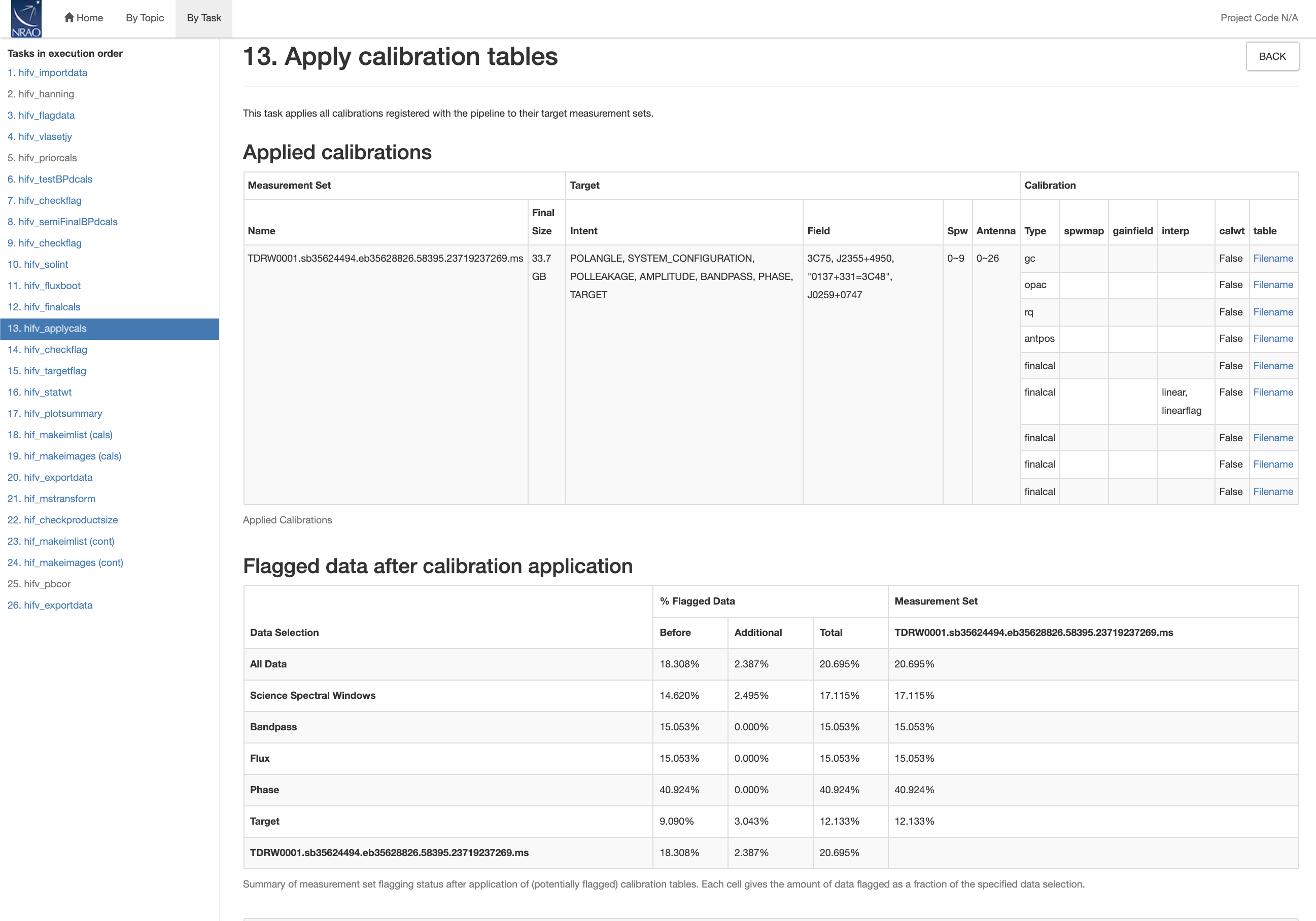 |
Note that this stage also shows the final MS file size after the creation of the additional MODEL and CORRECTED_DATA columns.
CHECK for: reasonable flagging statistics. If the flagging increased dramatically, some calibration tables should be examined for proper solutions.
QA: determined by the percentage of incremental flagging where 0 < score < 1 is the score range for 60% < fraction flagged data < 5%.
Stage 14. hifv_checkflag: Flag RFI on target using rflag
The rflag and tfcrop heuristics are now applied to the target to prepare it for imaging (Fig. 30).
 |
CHECK FOR: RFI removal in the target data through the diagnostic plots and data statistics. FOR SPECTRAL LINE DATA: do not run this step unless a cont.dat file is provided (c.f. the VLA Pipeline Webpage at http://go.nrao.edu/vla-pipe). Otherwise the spectral lines may be flagged, too.
QA: determined by the percentage of incremental flagging where 0 < score < 1 is the score range for 60% < fraction flagged data < 5%.
Stage 15. hifv_targetflag: Targetflag
The flagdata automated flagging routine rflag is run one more time with slightly different heuristics on all sources to remove additional RFI and other outliers from the data.
CHECK for: RFI removal in the target data (use plotms). Although flagging is performed for all fields, any additional flags have no more influence on the calibration tables because the calibration was applied in a previous stage. Flagging may, however, improve all images that are made in the following stages. In particular, the target fields are flagged here for the first time which will benefit their image quality. FOR SPECTRAL LINE DATA: do not run this step unless a cont.dat file is provided (c.f. the VLA Pipeline Webpage at http://go.nrao.edu/vla-pipe). Otherwise the spectral lines may be flagged, too.
QA: determined by the percentage of incremental flagging where 0 < score < 1 is the score range for 60% < fraction flagged data < 5%.
Stage 16. hifv_statwt: Reweighting visibilities
Since the VLA pipeline is currently not using the switched power calibration, there can be some sensitivity variations of the data over time due to changes in opacity, elevation, temperature (gradients) of the antennas, etc. It is usually advisable to weigh the data according to the inverse of the square of their noise. This is done via the CASA task statwt and will increase the signal-to-noise ratio of images. It might be worth going to the casa log that is linked on this page and check the variance and mean of the weights. If the variance is more than 100 times larger than the mean, then something is likely wrong and the data should be inspected further.
Note that features such as RFI spikes and spectral lines will influence RMS calculations and usually result in down-weighting data that includes such features.
CHECK for: mean and variance of the weights. Also: images that are created later should improve in their signal-to-noise. FOR SPECTRAL LINE DATA: do not run this step as spectral lines may be weighted down unless a cont.dat file is provided (cf the VLA Pipeline Webpage at http://go.nrao.edu/vla-pipe).
QA: N/A
Stage 17. hifv_plotsummary: VLA Plot Summary
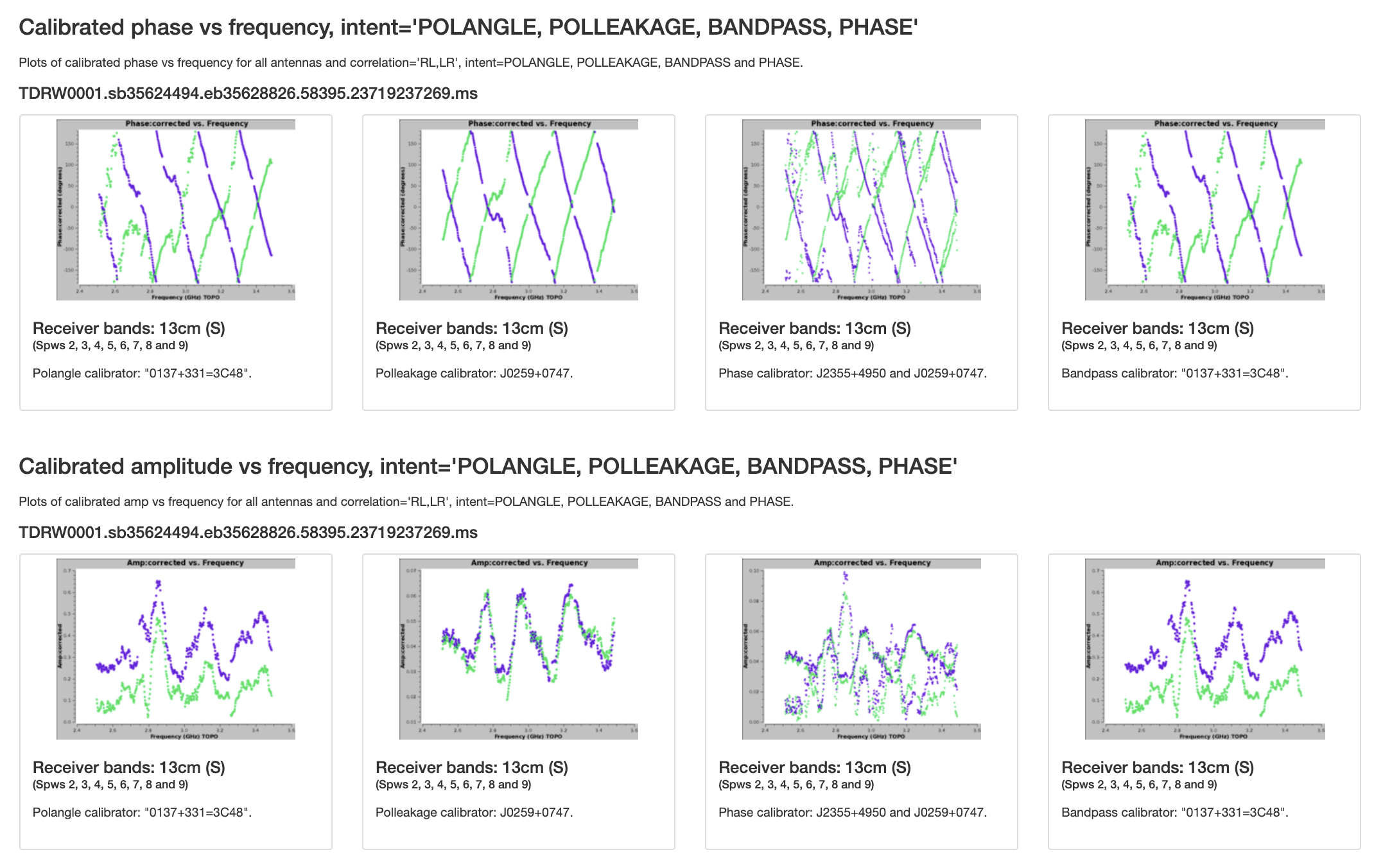
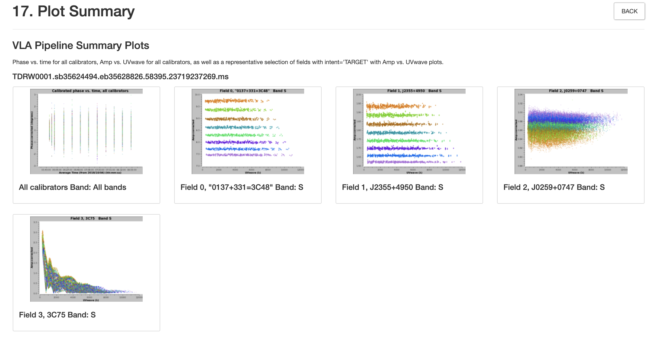
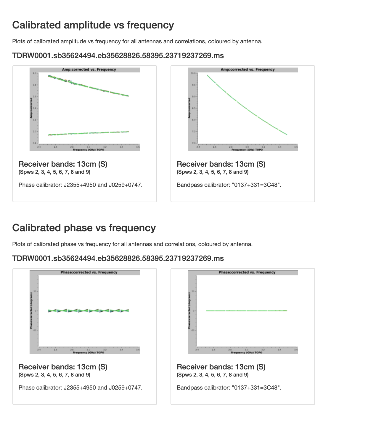
This task produces diagnostic plots of the final, calibrated data. These include: calibrated phase as a function of time for all calibrators, and amplitudes as a function of UVwave (UVdistance) for all science fields (incl. calibrators; Fig 31a); the amplitudes and phases as a function of frequency for the bandpass and phase calibrator(s) colored by antenna (Fig. 31b); amplitude against frequency for all science targets, colorized by spw (Fig. 31c); and phases as a function of time for all cross-hands (RL, LR) of the polarization calibrators (Fig. 31d).
The phases for all calibrators should be around zero. A large scatter like at 5:50 UT (first plot in Fig. 31a) should be inspected and could indicate that more flagging is required. We have already identified scans at this time range to show some problems in some antennas (e.g. ea01 and ea02; cf. Fig. 28a). Point sources with a flat spectral index should show up in the UVwave plots as straight, horizontal lines. The offset between the colored spws shows the spectral index of the sources.
The phases and amplitudes as a function of frequency for the phase calibrator overall look fine. Some scatter could be flagged and calibrated again, but if the scatter is symmetric, then the calibration table may still have good solutions. The zig-zag pattern of the phases is due to a small mismatch in the delay measurement timing (also known as 'delay clunking'). This is an internally generated effect. Typically the effect is averaged out over time.
 |
 |
The amplitudes as a function of frequency for all targets can be used to identify RFI or other problems with the data. Structure is only expected for very strong target sources.
The pipeline does not perform polarization calibration. The CASA guide Polarization Calibration based on CASA pipeline (3C75) explains how to do this, and is based on the results from this pipeline run.
CHECK for: outliers, jumps, offsets, and excessive noise.
QA: N/A
Stage 18. hif_makeimlist (cals): Compile a list of cleaned images to be calculated
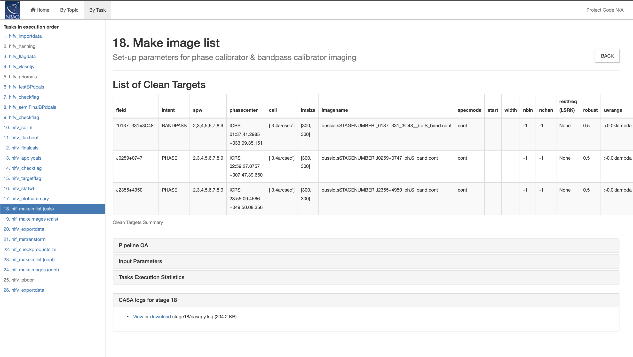
Finally, diagnostic images are made for each receiver frequency band by combining all covered spws for calibrators with a PHASE or BANDPASS intent (note that in our case the bandpass was derived from the FLUX calibrator as no BANDPASS intent was present). For each image, this stage calculates basic imaging parameters such as pixel resolution (cell size) and image sizes (cf. Fig. 32).
 |
This stage also issues warnings when spws are flagged entirely.
CHECK for: appropriate cell size for the images.
QA: N/A
Stage 19. hif_makeimages (cals): Calculate clean products
Based on the information from the previous hif_makeimlist stage, the images are now created by running the CASA task tclean and made available in the directory in which the pipeline was executed (usually where the SDM is located). Images are produced for each receiver frequency band using the multi-frequency synthesis algorithm, i.e. in continuum mode corrected for spectral dependencies using the stretched uv-coverage as sampled by the observed channel frequencies.
Image properties are provided for each image (Fig. 33). They contain beam characteristics as well as image statistics.
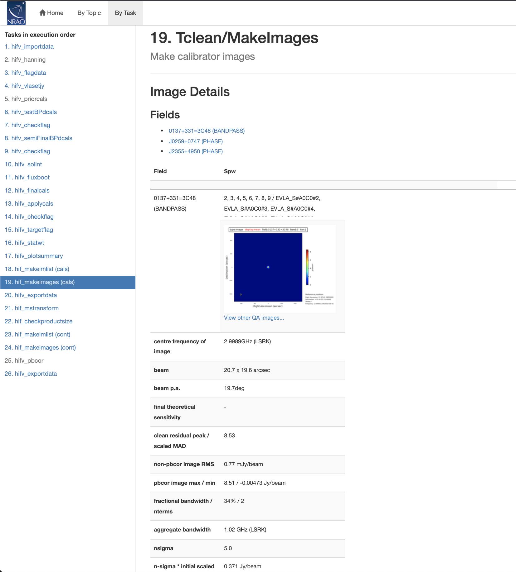 |
The full range of tclean products can be accessed by the link under the images: "View other QA images...". For the first field, an example is given in Fig. 34. The cleaning is performed in two stages, where the first stage is simply a dirty image, and the next iteration starts the actual deconvolution. For each iteration, the image and the residual are shown, together with a clean mask (here, the truncated primary beam). Other images on this page include the primary beam, the psf, and the final model.
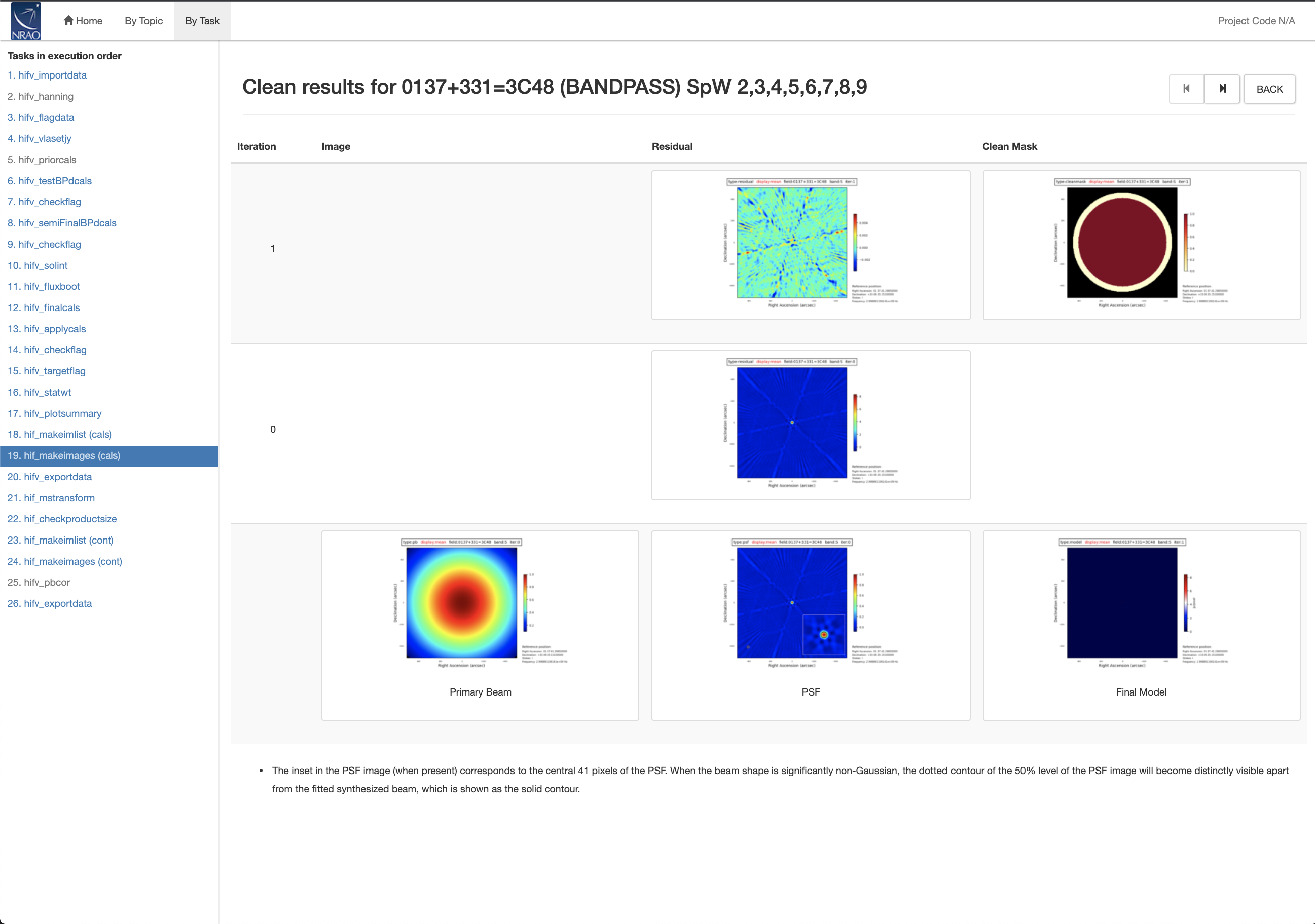 |
This step concludes the calibration pipeline.
CHECK for: degraded images, strong ripples, calibrators that do not resemble the point spread function (psf). Such images may indicate RFI or mis-calibrated sources.
QA: a linear score between 0 to 1 is assigned for signal to noise ratios between 5 and 100.
Stage 20. hif_exportdata: Create data products to be archived.
This stage is only shown for data that were run through the NRAO production pipeline and will usually not show up during manual execution of the pipeline. It provides information on the data products that will be available in the archive. Weblogs and calibration files are bundled and zipped in addition to the flags (Fig. 35). Images are converted to FITS format. More information on the files and the restoration process is provided on the VLA pipeline homepage.
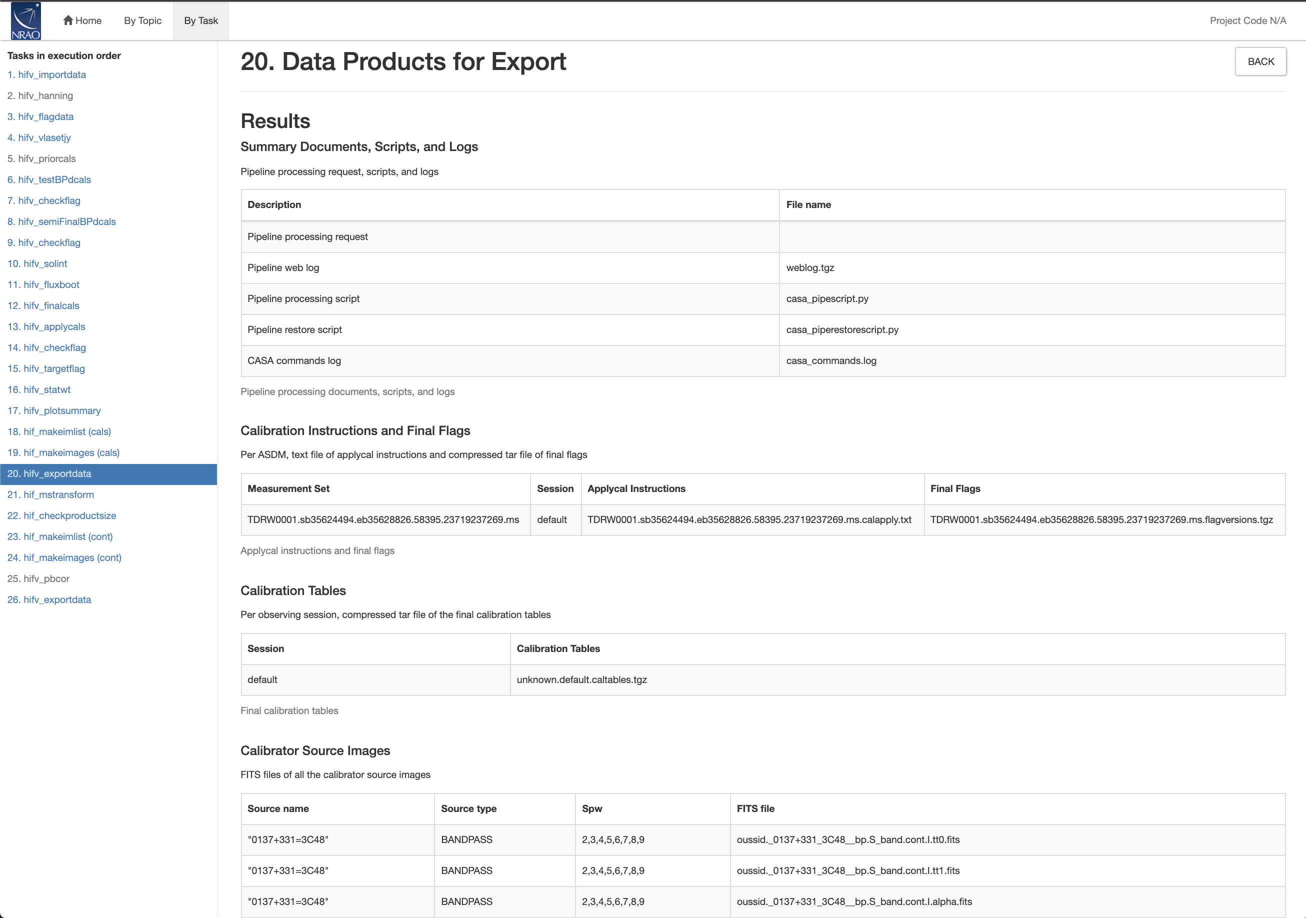 |
CHECK for: N/A
QA: N/A
Stage 21. hif_mstransform: Create MS for imaging.
This stage is the first step of the target imaging pipeline. All 'TARGET' scans are extracted from the parent MS and written into a new MS.
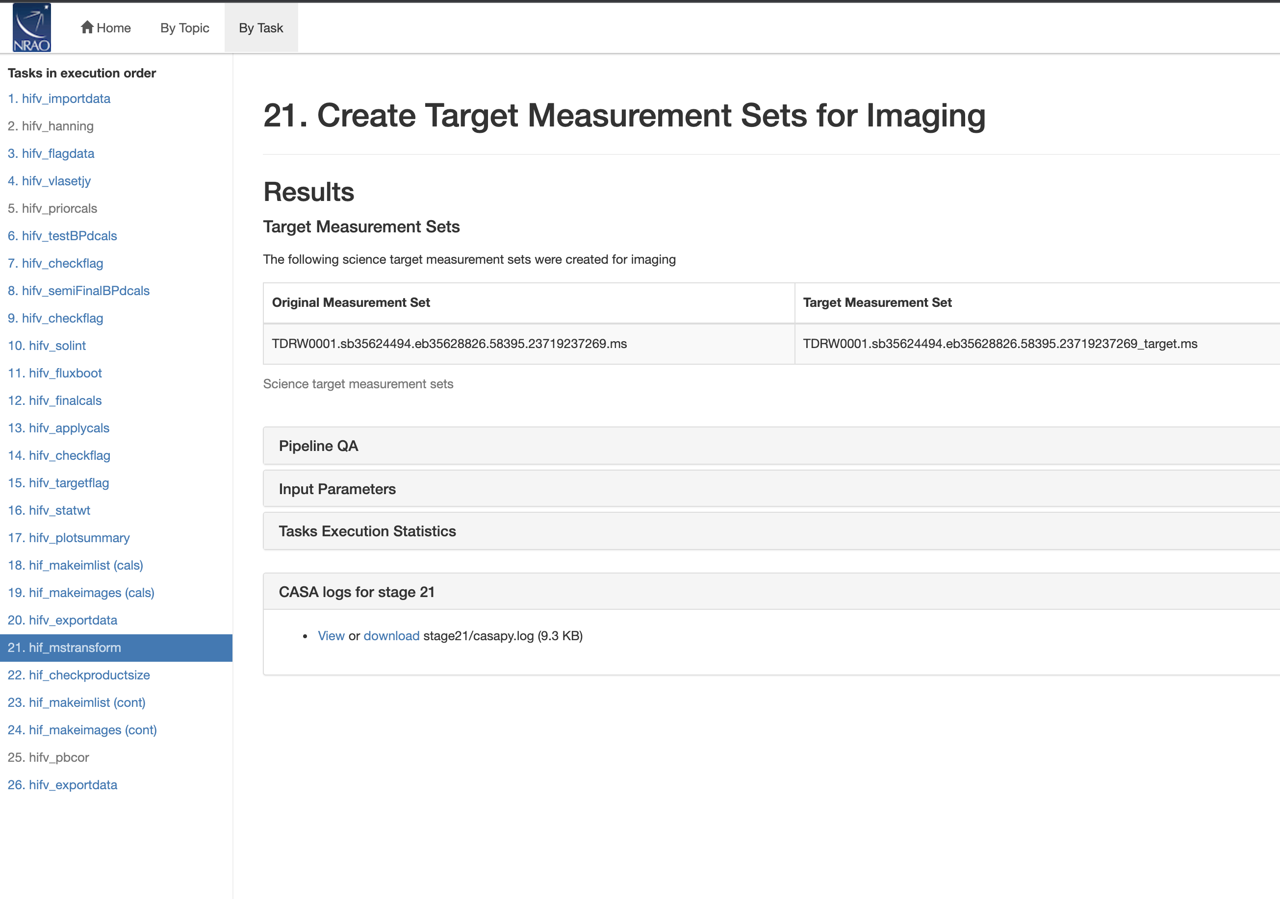 |
CHECK for: N/A
QA: N/A
Stage 22. hif_checkproductsize: Derive the size of the image products.
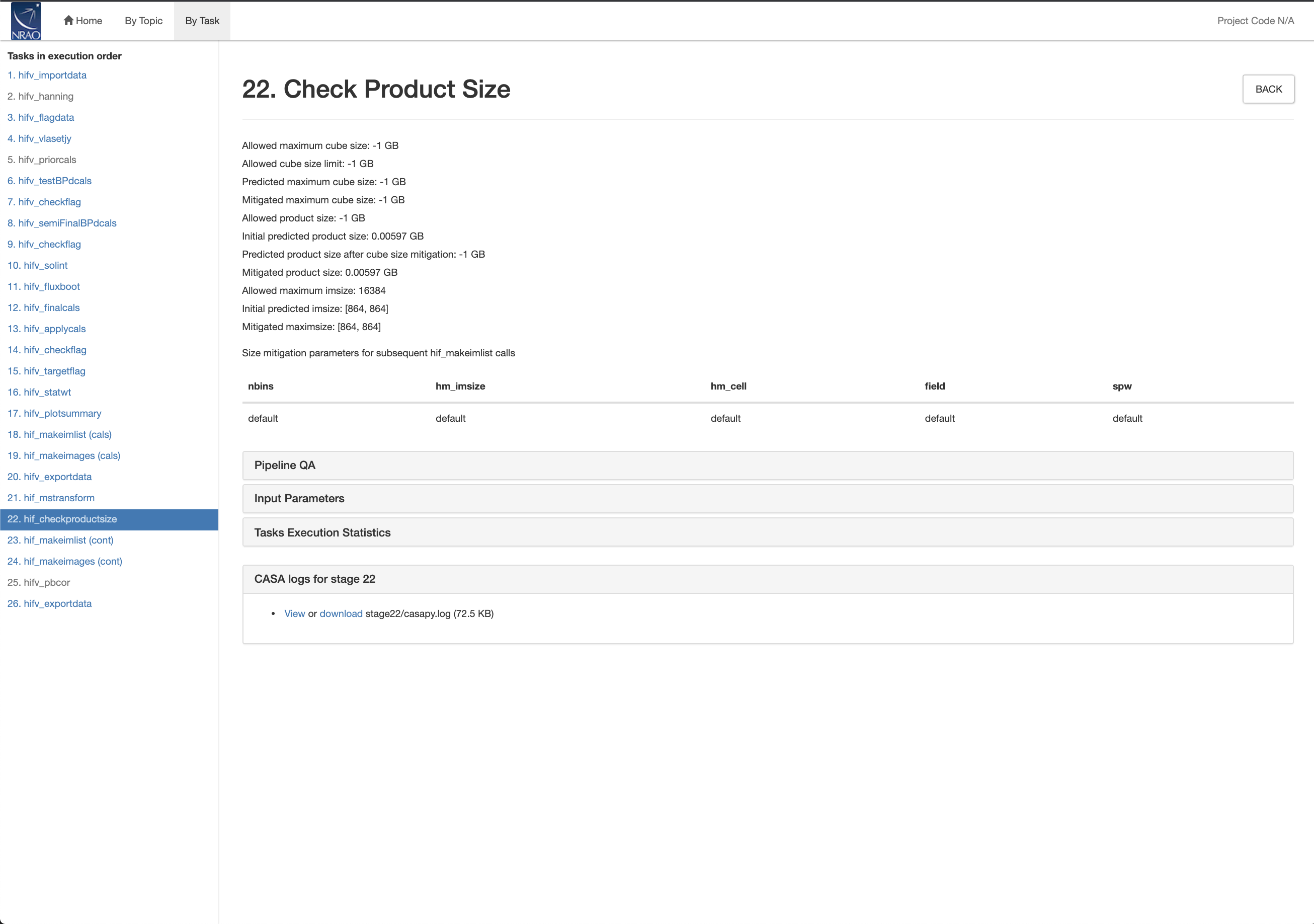
Before the target imaging starts, hif_checkproductsize will attempt to determine the optimum for cell size (based on the longest baseline), field of view (based on the primary beam), and number of spectral channels (in our case this is a single continuum channel). The scientifically ideal size of the image, however, may not always be practical and sometimes be too large. Settable parameters can limit the size of the image (cube). If the calculations exceed this limit, the image size will be reduced by increasing the cell size, decreasing the image size, or creating somewhat wider spectral channels (Fig. 37). The current, maximum size for continuum imaging is 16384x16384 pixels.
 |
CHECK for: Plausibility of the parameters, in particular when the task tries to adjust the optimal imaging parameters to match a size limit.
QA: N/A
Stage 23. hif_makeimlist (cont): Calculate and define the target imaging parameters.
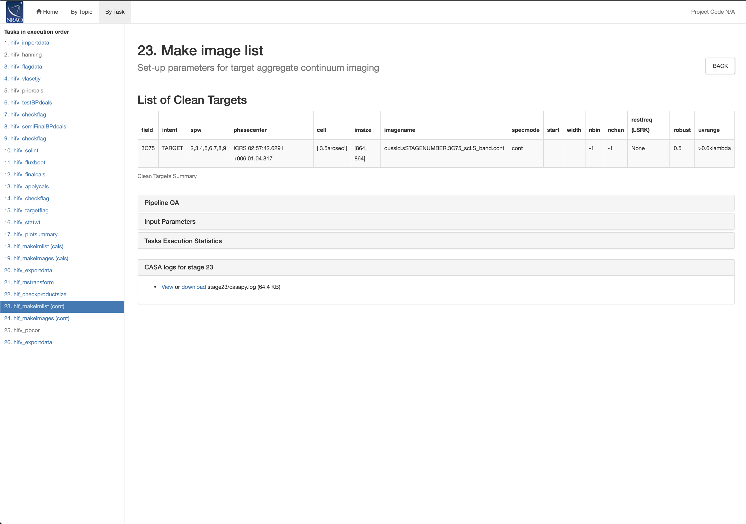
If the previous stage had limitations in the imaging parameters, they will now be used here. Otherwise, this stage itself is setting the parameters for the list of targets that will be imaged (Fig. 38). The image size aims to cover the inner primary beam for Ku and higher frequency and intends to reach the second null for X-band and lower (to include potential, bright sources that may still throw sidelobes into the main image). For A-configuration, though, images may be restricted by the 16384x16384 limit. Note that VLA Pipeline imaging only uses the standard gridder and is currently not applying special gridders like widefield or (a)w-projection.
 |
CHECK for: appropriate cell size for the images.
QA: N/A
Stage 24. hif_makeimages (cont): Create the target images.
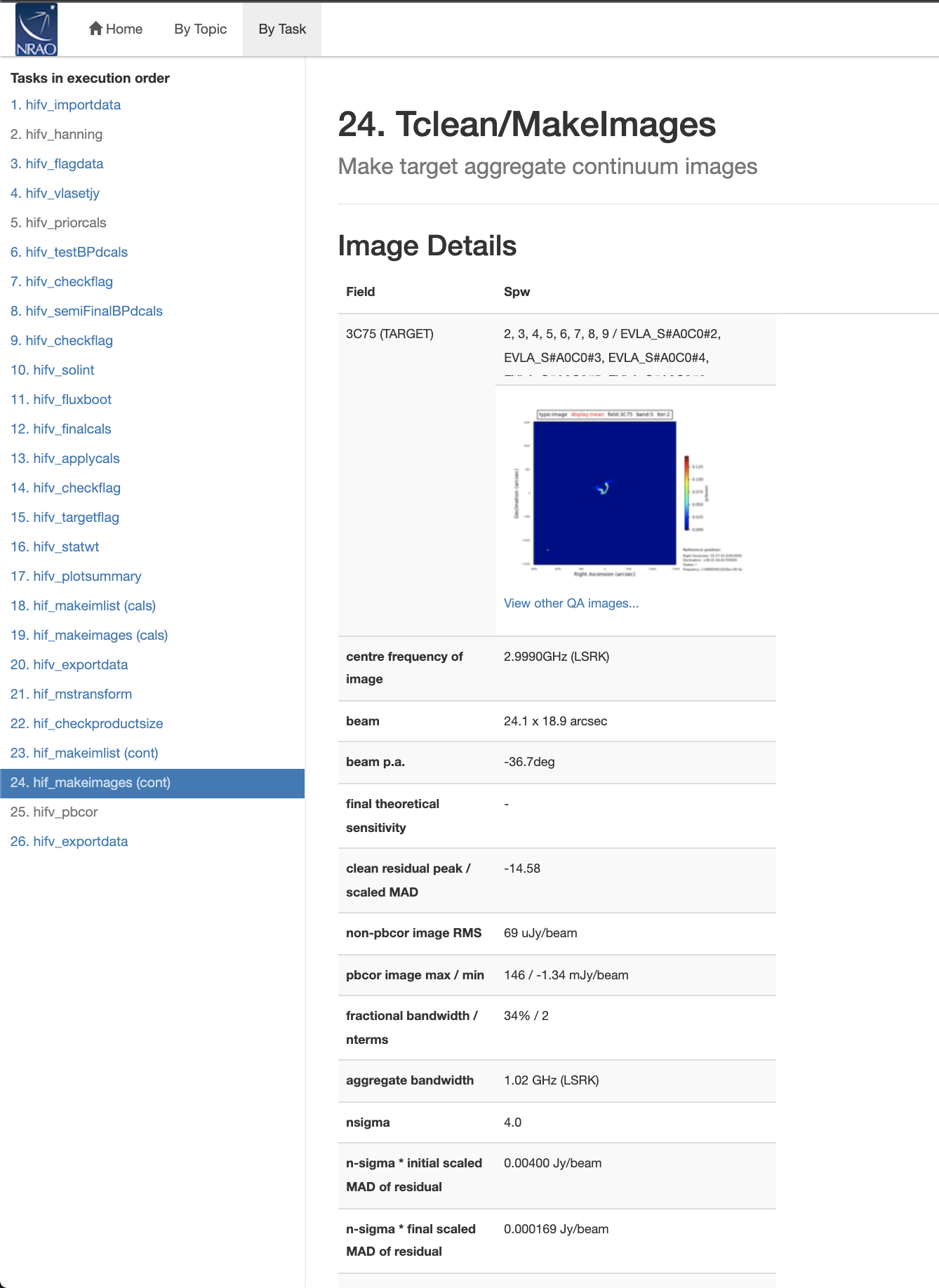
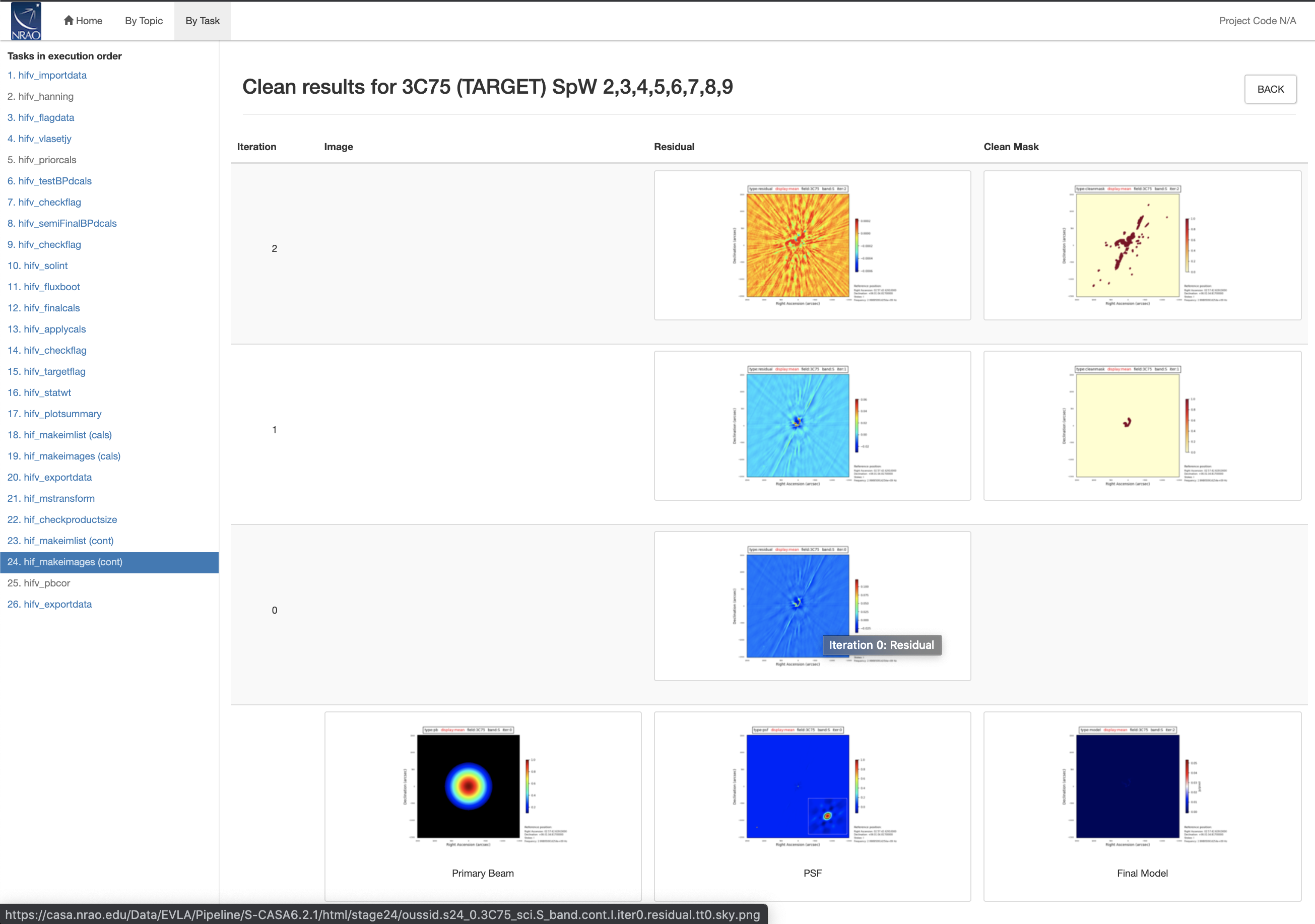
The target images are now created by CASA's tclean based on the previously determined imaging parameters. Image statistics and properties are provided here (Fig. 39). Additional imaging products are also available, similar to those in stage 19. Since the images are more complex, there are three stages now. The 0th stage is the creation of the dirty image, and the two subsequent stages include automasking procedures at two different cleaning depths (Fig. 40).
 |
 |
CHECK for: Image artifacts, missing short spacings, not fully deconvolved sources etc. The science target may be faint and not well shown in the weblog images. Use an image viewer to properly inspect the target image.
QA: N/A
Stage 25. hif_pbcor: Apply primary beam corrections.
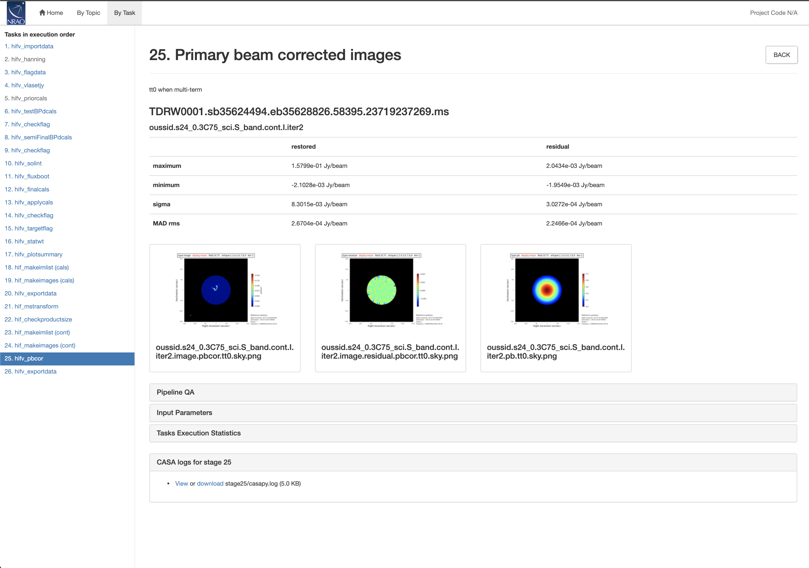
The Primary beam correction is applied in this stage that is separate from the imaging itself. Corrected images and residuals and new image statistics are displayed here (Fig. 41).
 |
CHECK for: N/A
QA: N/A
Stage 26. hif_exportdata: Accumulate and prepare data to be archived.
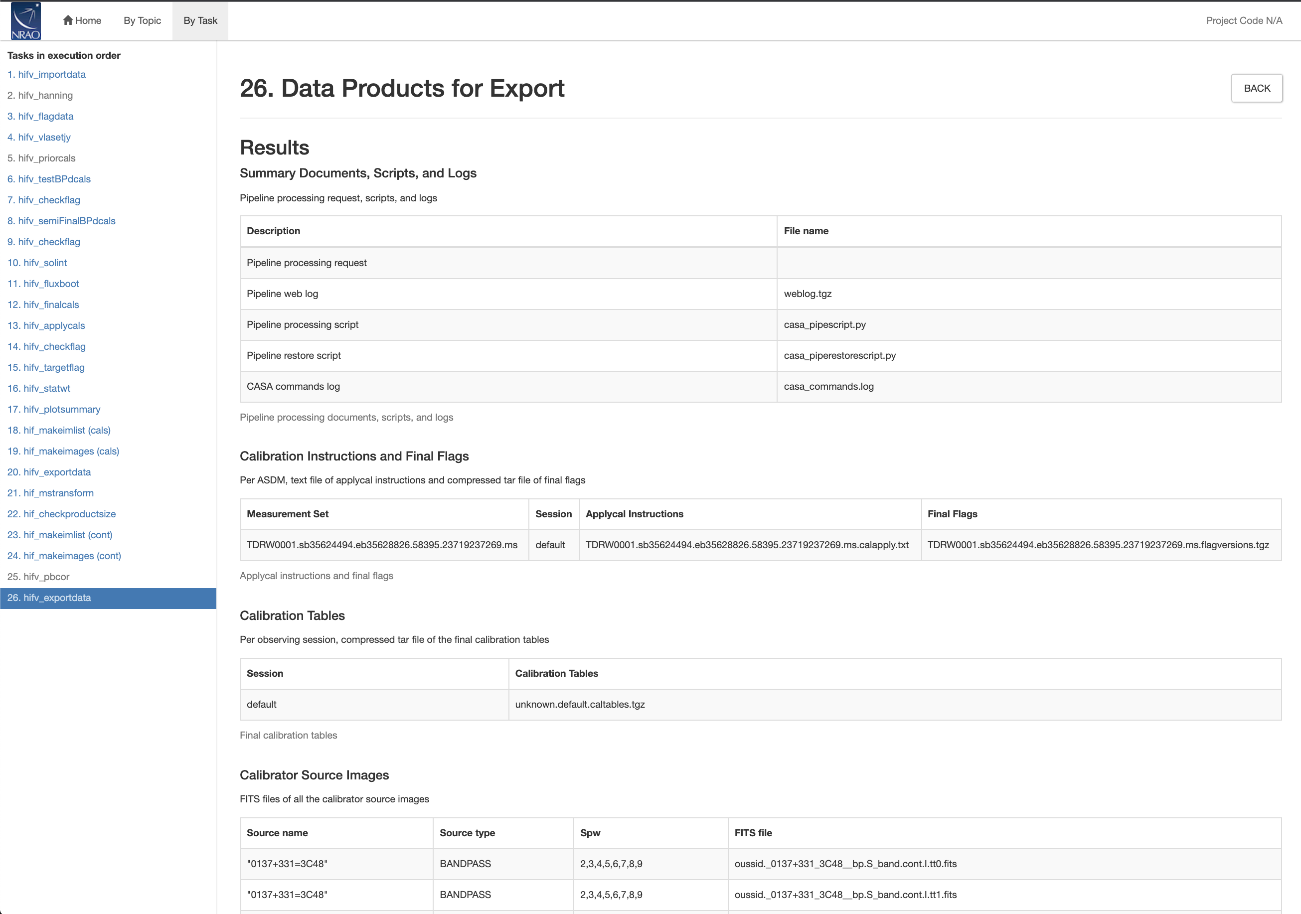
For NRAO processing this step collects and packages the pipeline results for storage in the NRAO archive (Fig. 42). This is not required but could also be useful for users.
 |
CHECK for: N/A
QA: N/A
Last checked on CASA Version 6.2.1

