Simalma (CASA 6.1.1)
This guide demonstrates how to use simalma, a CASA task that simplifies the process of simulating observations that combine data from the main 12 m array with data from the ALMA Compact Array (ACA) and total power (TP) antennas. The commands in this guide have been verified to work in CASA version 6.1.1. For CASA 6.1, the simalma task was improved to use tclean instead of the old clean for imaging. In addition, CASA 6.1.1 fixed a number of small bugs in simalma to ensure accurate scientific results (see CASA Docs). Those bug fixes are not available in CASA 6.1.2, 6.1.0, and earlier version, so please use CASA 6.1.1 for the simalma task where possible.
To learn how to create a script of the Python code on this page see Extracting scripts from these tutorials.
ALMA consists of the main array of 12m antennas plus the ACA, which includes an array of 7 m antennas and a separate set of 12 m antennas used for Total Power measurements. CASA enables users to simulate observations using any or all of these components.
Simulating Observations with the Main 12 m Array and the ACA: Manual Combination of the Data
One could simulate observations that use the main array plus the ACA by generating the data for each component separately and then "manually" combining and imaging the data. The approach is to use simobserve to generate simulated uv data sets for each component separately, and then combine and image the resulting Measurement Sets using simanalyze. This technique is general and can be used to simulate observations using multiple 12m array configurations, as well. Total power observations can be simulated either in an independent run of simobserve, or integrated with one of the interferometric simulations. Note that if you simulate total power and interferometric observations simultaneously with simobserve, they must have the same set of pointing centers and the same integration and total time. These are not realistic conditions. For example, to reduce edge effects, the Total Power antennas should observe a larger area on the sky than the main array antennas, by about 1/2 of a primary beam. So, it is generally better to generate the total power data with a separate run of simobserve.
This "manual" method of combining main-array data with ACA data is described in the ACA_Simulation_(CASA_5.4) guide.
The simalma task
The simalma task has been available in CASA since CASA version 4.1, but received an upgrade in CASA 6.1.1. This task takes one set of parameters describing the region of the sky to observe, and makes the appropriate calls to simobserve and simanalyze. Here we give an example showing how to use simalma.
Set simalma as current task
Reset all parameters to default, then set the project name to m51 and allow simalma to overwrite files
# Set simalma to default parameters
default("simalma")
# Our project name will be "m51", and all simulation products will be placed in a subdirectory "m51/"
project="m51"
overwrite=True
Specify sky model image
In this example, we'll use an Halpha image of M51 as the model of the sky. The curl command used below will copy a data file with the model image to our local disk and rename it.
# Model sky = Halpha image of M51
os.system('curl https://casaguides.nrao.edu/images/3/3f/M51ha.fits.txt -f -o M51ha.fits')
skymodel         =  "M51ha.fits"
Note that simalma will not modify your original input image. Rather, it will make a copy m51/m51.skymodel.
To make the M51 Halpha image more suitable to a sub-millimeter ALMA observation, we will modify most of the header parameters from the FITS file. We will:
- place the source in the southern hemisphere with the indirection parameter,
- set the pixel size to 0.1arcsec, to simulate an observation of a galaxy that is smaller in angular size than M51. (M51 itself would require a quite large mosaic, and in any case we'd like the angular scale of pixels in the input model to be significantly smaller than the synthesized beam.)
- set the peak brightness to 0.004 Jy/pixel
- set the center observing frequency to 330GHz, and since it's a 2D image we'll set the single "channel" width to be 50MHz. These parameters are plausible for observing a sub-mm emission line in a galaxy.
# Set model image parameters:
indirection="J2000 23h59m59.96s -34d59m59.50s"
incell="0.1arcsec"
inbright="0.004"
incenter="330.076GHz"
inwidth="50MHz"
Set up Observing Parameters, and Run

We will simulate observations using the main array in "configuration number 3" from Cycle 6. To that we will add the ACA cycle 6 array. This configuration affords ~0.5 arcsec resolution. Here is a list of configuration files available in CASA 6.1.
antennalist=["alma.cycle8.3.cfg","aca.cycle8.cfg"]
We'll set the 12m array observing time to 30 minutes:
totaltime="1800s"
The 7 m array observing time is set by default to be twice the 12 m Array time. So in this instance, the 7 m array will observe for 1 hour. The user can set this to a different value by entering the 12 m time and the 7 m time as a 2-element array in the totaltime parameter. See the CASA Docs documentation for simalma for details.
For this simulation we will also "single-dish" total power observations with two antennas from the 12 m Total Power Array. A typical observation with the Total Power Array will last 4 times the total time of the 12 m main array.
In CASA 5.4 simulations, the total power observations are simulated in a single track. So the total time of a TP observations should be roughly 8 hours or less, depending on the target declination, to ensure that the target position remains above the horizon. Until this limitation is addressed in a future CASA release, you should limit simulations that include the TP Array to short total integration times.
tpnant = 2
tptime="7200s"
We set the precipitable water vapor to 0.6 mm to represent observations in nominal weather. The simulation will add noise to the data based on this setting.
pwv=0.6
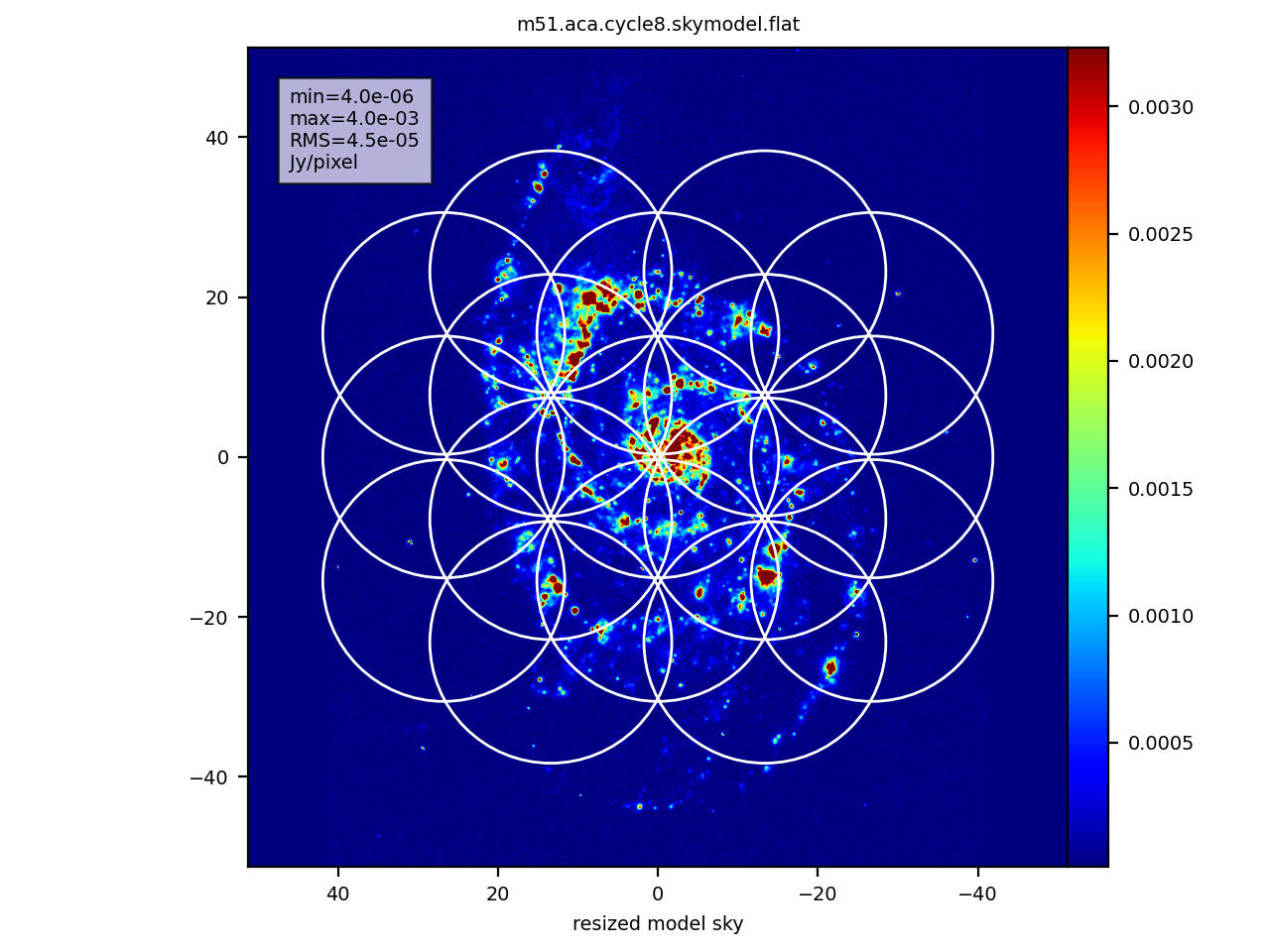
To cover all of the galaxy according to our rescaled pixel size, we will need a 1 arcmin mosaic, and we will let simalma calculate the pointings for us:
mapsize="1arcmin"
We also set the number of iterations for cleaning of the signal (deconvolution and restoration) to 100
niter=100
Finally you can check the input settings and run the simulation.
dryrun = False
inp
go
What does simalma do?

Generate visibilities and images for each array
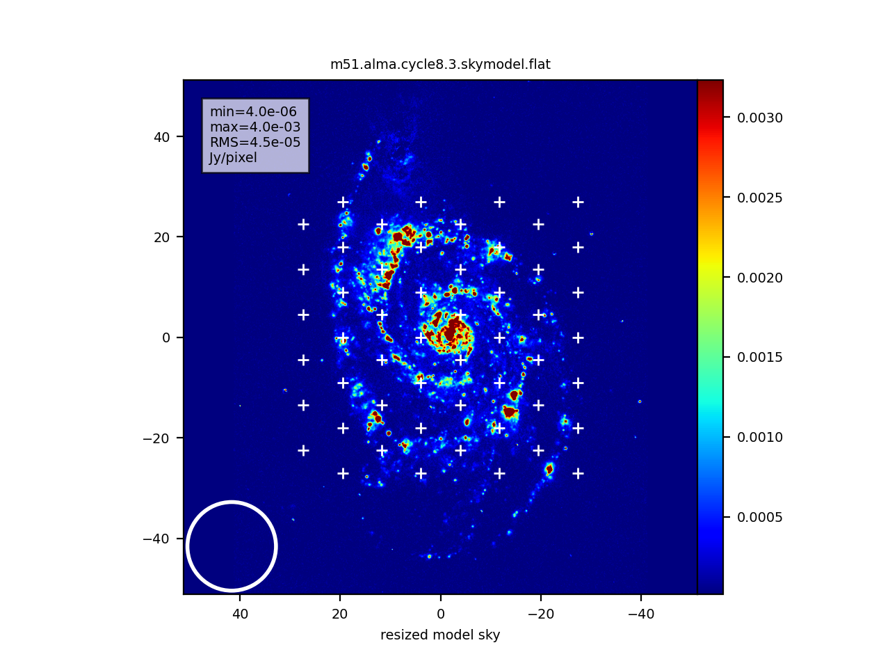
The simalma task first calls simobserve to simulate the visibilities for each of the three array components: the 12 m Main Array, the 7 m Array, and the 12 m Total Power Array. The simobserve task generates a figure showing the elevation of the target, the antenna layout, the uv coverage, and the synthesized dirty beam.
Next simalma generates an image from each of the three array components, separately. This step is not essential to getting the final result from the combined arrays, but it provides a useful diagnostic. The images will be named according to the antennalist parameter above. For example, the ALMA 12m image is called m51.alma.cycle8.3.noisy.image.

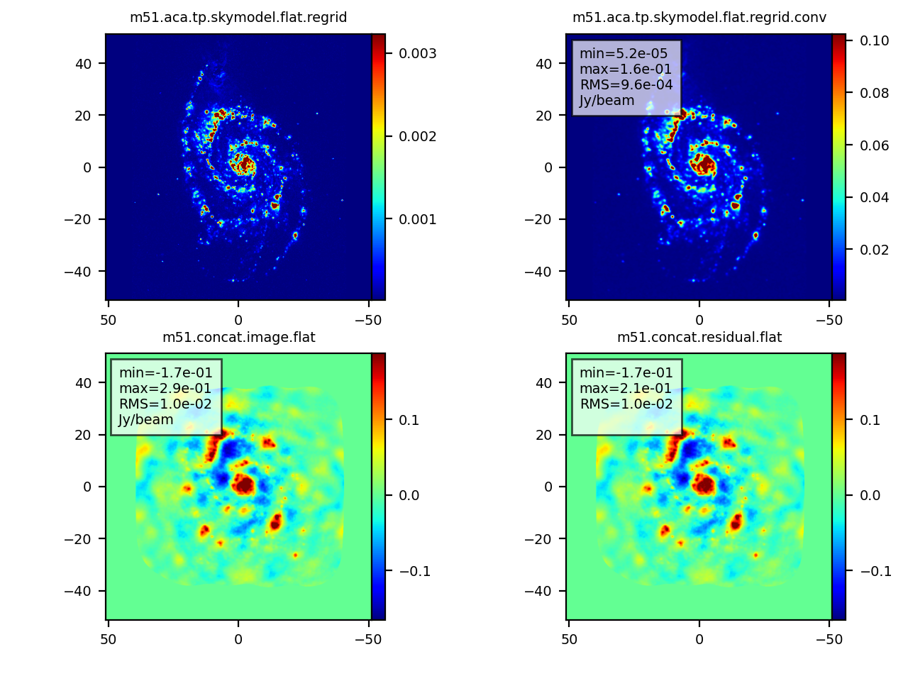
It is useful to know that simalma generates a version of the input sky model convolved to the ACA resolution. In this example it is called m51.aca.tp.cycle8.skymodel.flat.regrid.conv. That image can be useful to better understand the simulation results.
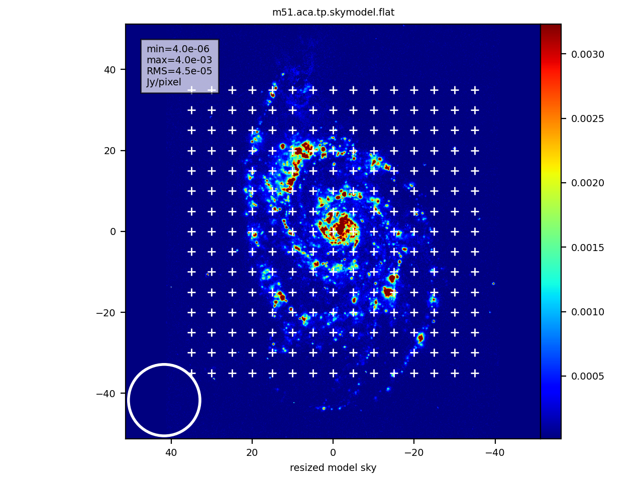
Note that the total power map covers the same region as the main array mosaic, with an extra pointing position added around the outside edge of the map so that the total power map is larger than the interferometric mosaic. (Total power maps usually have additional noise and artifacts at their edges). Furthermore, a square raster pattern is used instead of the hexagonal pattern of the interferometric array maps.

Combine the UV data from the 3 components and make the final image
Next simalma uses simanalyze to combine the three measurement sets and create a single image. It accomplishes this in the following manner.
First, simalma concatenates the two sets of interferometric visibilities, and images them. Diagnostic graphics with "concat" in their names are generated:

Finally it combines the total power image with the concatenated interferometric image using the CASA task feather.
Note, there are many ways to combine data from separate observations. If you are dealing with real ALMA data, you may wish to discuss options with scientists at your ARC.
Some notes for combining data "manually"
- When combining interferometric data from different arrays "manually", it is critical to set the relative data weights properly. Simulated data have weights=1, since the thermal noise is generated uniformly per baseline. However, in reality the 7m baselines have lower sensitivity than the 12m baselines, and their weights must be decreased by the sensitivity ratio. simalma uses the visweightscale parameter of concat to apply that lower weight of (7/12)**2 to the 7m visibilities. If you wish to combine data manually, you must do this step yourself.
- When combining the single dish and interferometric maps in the image plane using the feather task, one must use the interferometric map without the primary beam correction, and first multiply the total power map by the interferometric sensitivity image (".flux") -- this ensures that noise effects are properly handled on the edges of each map. After running feather, the output is masked to 0.2 times the interferometric primary beam, since the total power map was created larger than the interferometric map on purpose, so the edges of the combined image do not contain any interferometric information.:
