MG0414+0534 P-band Spectral Line Tutorial - CASA 6.5.2
This CASA Guide is for Version 6.5.2 of CASA.
| DISCLAIMER |
| The following guide is for users who are experts in data reduction using CASA. If you are a beginner or novice user, please review other CASA guides found at VLA Tutorials. Note: This guide may take up to 2-days to complete |
Overview
This tutorial describes how to use CASA 6.5.2 to reduce spectral-line data in the low-frequency P-band of the VLA (230–470 MHz). The goal is to make an image cube containing HI 21cm absorption against the strong radio continuum of gravitationally lensed radio galaxy MG0414+0534. As a result of the high redshift of z=2.6365, the HI absorption signal in MG0414+0534 is redshifted to an observed frequency of 390.597 MHz. The HI absorption in MG0414+0534 was previously imaged with the VLA by Moore, Carilli & Menten 1999 (ApJ, 510, 87), before the upgrade to the WIDAR system.
We would like to note that the CASAviewer (supporting tasks viewer, imview and msview) has not been maintained for a few years now and will be removed from future versions of CASA. The NRAO replacement visualization tool for images and cubes is CARTA, the “Cube Analysis and Rendering Tool for Astronomy”. It is available from the CARTA website. We strongly recommend to use CARTA, as it provides a much more efficient, stable, and feature rich user experience. A comparison of the CASAviewer and CARTA, as well as instructions on how to use CARTA at NRAO is provided in the respective section of the CASA docs. This tutorial shows Figures generated with CARTA for visualization.
Observing strategy
To perform P-band spectrsocopy, there are three important considerations for planning the observations:
- Use a bandpass calibrator that is strong enough to accurately calibrate the frequency-dependent gain variations. This is particularly important for most HI 21cm absorption projects, which are typically performed against strong radio continuum sources. As a rule-of-thumb, use tcal > tobj × (Sobj / Scal)2, with t the exposure time and S the source flux density. This rule-of-thumb serves to avoid introducing excessive additional noise in the spectrum.
- Additionally, if very high spectral dynamic range is needed (i.e., when expecting a ratio between the detection limit and the radio continuum of about 1:10,000 or more), consider observing a bandpass calibrator several times during your run to be able to correct for time-varying bandpass changes, which scale with the continuum emission in the target field. See the Calibration section of the Guide to Observing with the VLA for more information.
- Use a bandwidth that is wide enough to perform accurate self calibration. Using a wide bandwidth for self-calibration is important for fields with relatively weak continuum sources. For strong continuum sources, a narrower bandwidth can be used to avoid excessive RFI.
The P-band test data on MG0414+0534 that we use in this tutorial were obtained using a large bandwidth. This is to ensure that good bandpass solutions can be procured, and that self-calibration can accurately be performed. However, due to the strong radio continuum of MG0414+0534 (3.3 Jy at 390 MHz), and the large amounts of RFI across the entire band, we only use a small fraction of the total band for data reduction and analysis in this tutorial.
Obtaining the data
This 33 GB data set can be downloaded by clicking here. The filename should be MG0414_d1_data.ms.tgz (add the ".tgz" if this is missing). We are providing this starting data set, rather than the original data set for two reasons. First, many of these initial processing steps can be rather time consuming (> 1 hr). Second, while necessary, many of these steps are not fundamental to the calibration and imaging process, which is the focus of this tutorial. We will use test data that was taken in a hybrid configuration when the VLA array was being moved from B-config to A-config.
The entire data set can be downloaded from the NRAO archive by searching for the following Project Code:
TSUB0001
This returns a long list with test-data that are publicly available. Our observations were performed on 14 Sept 2016:
TSUB0001.sb32720781.eb32763188.57645.263958564814
Note that this observation was duplicated on 15 September 2016.
The 15 GB data set from the download has already had online flagging and Hanning smoothing applied, and the smaller data set split out from the larger data set. If you wish, you can download the SDM from the NRAO archive in order to apply the online flags and run Hanning smoothing on the large data set before splitting out the smaller data set to work on. To apply the on line flag use the task flagcmd; to apply the Hanning smoothing use the task hanningsmooth on scans 7 to 16 and field 3 and 4; and to split the data, use the task split. For the purpose of this tutorial, we only reduce and image the first data set. Then, you will need to split only the spw 17, and only channels 20 to 485 to remove the borders.
Examining the Data
Loading data into CASA
We will have to untar the 15 GB data set that you've downloaded.
# in a terminal, outside of CASA:
tar -xzf MG0414_d1_data.ms.tgz
Please use CASA 6.5.2 for this tutorial (typing casa -ls in a linux window shows the available versions and the current version; to explicitly change the version type, e.g., casa -r 6.5.2-26-py3.6)
casa
on the command line. This should start a CASA interactive python (iPython) session, and open a separate log window. To guarantee that the below mentioned procedure for data reduction and imaging works, make sure you are using CASA version 6.5.2. While older versions may work as well for the purpose of this tutorial, it is good to read instructions on how to download and install the latest version of CASA.
It is a good practice to read the Operator Log that was created by the duty operator during the observations. This log can provide additional information on data that should be flagged manually during the data reduction stage. The Operator logs can be found at Ops Logs form entry, and this is the direct link for the log of the observation (in PDF format).
Inspecting the observation info
We will inspect the content of our data set using CASA task listobs.
# In CASA
listobs(vis='MG0414_d1_data.ms')
The task plots an overview of the data in the CASA logger. Notice that the task returns a dictionary on the terminal screen. Using the parameter listfile=`listobs.txt’, this information is written out to the file listobs.txt:
# In CASA
listobs(vis='MG0414_d1_data.ms', listfile='listobs.txt')
The content is included below:
   Observer: . Frazer Owen     Project: uid://evla/pdb/1695465
Observation: EVLA
Data records: 1179738       Total elapsed time = 9390 seconds
   Observed from   14-Sep-2016/06:43:48.0   to   14-Sep-2016/09:20:18.0 (UTC)

   ObservationID = 0         ArrayID = 0
  Date        Timerange (UTC)          Scan  FldId FieldName             nRows     SpwIds   Average Interval(s)    ScanIntent
  14-Sep-2016/06:43:48.0 - 06:48:42.0     7      0 3C48                     37044  [0]  [3] [CALIBRATE_AMPLI#UNSPECIFIED,CALIBRATE_BANDPASS#UNSPECIFIED,CALIBRATE_FLUX#UNSPECIFIED,CALIBRATE_PHASE#UNSPECIFIED]
              06:48:45.0 - 07:08:39.0     8      1 MG0414+0534             150444  [0]  [3] [OBSERVE_TARGET#UNSPECIFIED]
              07:08:42.0 - 07:28:36.0     9      1 MG0414+0534             150444  [0]  [3] [OBSERVE_TARGET#UNSPECIFIED]
              07:28:39.0 - 07:48:33.0    10      1 MG0414+0534             150444  [0]  [3] [OBSERVE_TARGET#UNSPECIFIED]
              07:48:36.0 - 08:08:30.0    11      1 MG0414+0534             150444  [0]  [3] [OBSERVE_TARGET#UNSPECIFIED]
              08:08:33.0 - 08:14:30.0    12      0 3C48                     44982  [0]  [3] [CALIBRATE_AMPLI#UNSPECIFIED,CALIBRATE_BANDPASS#UNSPECIFIED,CALIBRATE_FLUX#UNSPECIFIED,CALIBRATE_PHASE#UNSPECIFIED]
              08:14:33.0 - 08:34:27.0    13      1 MG0414+0534             150444  [0]  [3] [OBSERVE_TARGET#UNSPECIFIED]
              08:34:30.0 - 08:54:21.0    14      1 MG0414+0534             150066  [0]  [3] [OBSERVE_TARGET#UNSPECIFIED]
              08:54:24.0 - 09:14:18.0    15      1 MG0414+0534             150444  [0]  [3] [OBSERVE_TARGET#UNSPECIFIED]
              09:14:21.0 - 09:20:18.0    16      0 3C48                     44982  [0]  [3] [CALIBRATE_AMPLI#UNSPECIFIED,CALIBRATE_BANDPASS#UNSPECIFIED,CALIBRATE_FLUX#UNSPECIFIED,CALIBRATE_PHASE#UNSPECIFIED]
           (nRows = Total number of rows per scan)
Fields: 2
  ID   Code Name                RA               Decl           Epoch   SrcId      nRows
  0    NONE 3C48                01:37:41.299431 +33.09.35.13299 J2000   0         127008
  1    NONE MG0414+0534         04:14:37.800000 +05.34.41.99999 J2000   1        1052730
Spectral Windows:  (1 unique spectral windows and 1 unique polarization setups)
  SpwID  Name           #Chans   Frame   Ch0(MHz)  ChanWid(kHz)  TotBW(kHz) CtrFreq(MHz) BBC Num  Corrs
  0      EVLA_P#A0C0#17    466   TOPO     386.312        15.625      7281.2    389.9453       12  XX  XY  YX  YY
Sources: 2
  ID   Name                SpwId RestFreq(MHz)  SysVel(km/s)
  0    3C48                0     -              -
  1    MG0414+0534         0     -              -
Antennas: 27:
  ID   Name  Station   Diam.    Long.         Lat.                Offset from array center (m)                ITRF Geocentric coordinates (m)
                                                                     East         North     Elevation               x               y               z
  0    ea01  W24       25.0 m   -107.38.49.0  +33.53.04.0      -2673.3457    -1784.6009       10.4844 -1604008.744400 -5042135.825100  3553403.710800
  1    ea02  W56       25.0 m   -107.44.26.7  +33.49.54.6     -11333.1991    -7637.6832       15.3636 -1613255.391400 -5042613.097800  3548545.906000
  2    ea03  W40       25.0 m   -107.41.13.5  +33.51.43.1      -6377.9680    -4286.7773        8.2312 -1607962.451800 -5042338.218100  3551324.962400
  3    ea04  E04       25.0 m   -107.37.00.8  +33.53.59.7        102.7973      -63.7800       -2.6177 -1601068.806000 -5042051.932700  3554824.838800
  4    ea05  E36       25.0 m   -107.33.20.2  +33.52.34.3       5761.3733    -2704.6731       33.0133 -1596127.730800 -5045193.742100  3552652.419700
  5    ea06  N24       25.0 m   -107.37.16.1  +33.55.37.7       -290.3584     2961.8653      -12.2425 -1600930.069900 -5040316.395500  3557330.390000
  6    ea07  N16       25.0 m   -107.37.10.9  +33.54.48.0       -155.8512     1426.6377       -9.3934 -1601061.954400 -5041175.875300  3556058.026700
  7    ea08  W64       25.0 m   -107.46.20.1  +33.48.50.9     -14240.7524    -9606.2900       17.0885 -1616361.575500 -5042770.516600  3546911.419900
  8    ea09  N40       25.0 m   -107.37.29.5  +33.57.44.4       -633.6056     6878.5897      -20.7984 -1600592.749000 -5038121.341300  3560574.826900
  9    ea10  E20       25.0 m   -107.35.43.6  +33.53.29.9       2082.1759     -987.0087        9.4361 -1599340.800100 -5043150.963000  3554065.231500
  10   ea12  N32       25.0 m   -107.37.22.0  +33.56.33.6       -441.7248     4689.9674      -16.9328 -1600781.044500 -5039347.439100  3558761.527100
  11   ea13  E28       25.0 m   -107.34.39.3  +33.53.04.9       3732.7776    -1757.3308       21.4271 -1597899.895900 -5044068.684700  3553432.450200
  12   ea14  E08       25.0 m   -107.36.48.9  +33.53.55.1        407.8283     -206.0315       -3.2236 -1600801.931400 -5042219.382600  3554706.429400
  13   ea15  N64       25.0 m   -107.37.58.7  +34.02.20.5      -1382.3871    15410.1326      -40.6450 -1599855.687000 -5033332.368600  3567636.606800
  14   ea16  W72       25.0 m   -107.48.24.0  +33.47.41.2     -17419.4641   -11760.2694       14.9442 -1619757.299900 -5042937.656400  3545120.392300
  15   ea17  N56       25.0 m   -107.37.47.9  +34.00.38.4      -1105.2042    12254.2800      -34.2710 -1600128.378100 -5035104.139200  3565024.633900
  16   ea18  W48       25.0 m   -107.42.44.3  +33.50.52.1      -8707.9181    -5861.7682       15.5302 -1610451.901900 -5042471.123800  3550021.073100
  17   ea19  W16       25.0 m   -107.37.57.4  +33.53.33.0      -1348.7121     -890.6209        1.2959 -1602592.853500 -5042054.992400  3554140.702800
  18   ea20  E16       25.0 m   -107.36.09.8  +33.53.40.0       1410.0403     -673.4656       -0.7790 -1599926.104100 -5042772.977200  3554319.801100
  19   ea21  E24       25.0 m   -107.35.13.4  +33.53.18.1       2858.1906    -1349.1352       13.7186 -1598663.082000 -5043581.391200  3553767.014100
  20   ea22  W32       25.0 m   -107.39.54.8  +33.52.27.2      -4359.4399    -2923.1314       11.7614 -1605808.634100 -5042230.084000  3552459.197800
  21   ea23  E12       25.0 m   -107.36.31.7  +33.53.48.5        848.6994     -411.6226       -2.7575 -1600416.518000 -5042462.430500  3554536.041700
  22   ea24  W08       25.0 m   -107.37.21.6  +33.53.53.0       -432.1080     -272.1514       -1.5061 -1601614.083200 -5042001.656900  3554652.505900
  23   ea25  N08       25.0 m   -107.37.07.5  +33.54.15.8        -68.9088      433.1829       -5.0674 -1601147.942500 -5041733.833600  3555235.947000
  24   ea26  E32       25.0 m   -107.34.01.5  +33.52.50.3       4701.6503    -2209.7119       25.1976 -1597053.124400 -5044604.675000  3553058.992700
  25   ea27  N48       25.0 m   -107.37.38.1  +33.59.06.2       -855.2719     9405.9407      -25.9485 -1600374.881000 -5036704.201700  3562667.858900
  26   ea28  N72       25.0 m   -107.38.10.5  +34.04.12.2      -1685.6797    18861.8306      -43.5015 -1599557.928700 -5031396.353400  3570494.736800
 |
 |
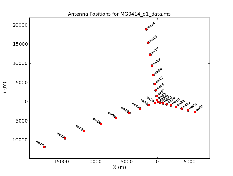
| Figure 1a. Plotants plot for MG0414. |
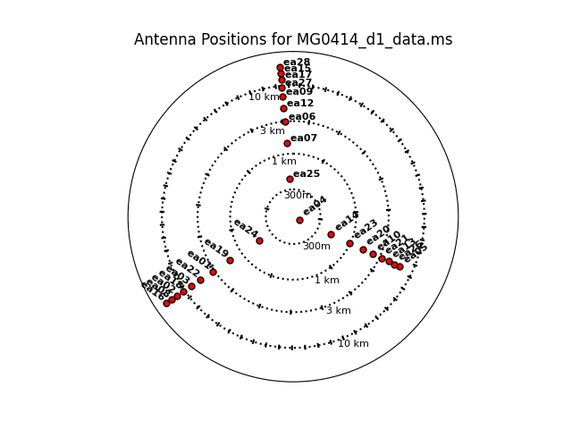
Figure 1b. Plotants plot for MG0414 in a log scale. |
Next we look at a graphical plot of the antenna locations and save a hard copy in case you want it later using CASA task plotant (see Figures 1a and 1b). This will be useful for selecting a reference antenna. Note that the VLA was in a period of re-configuration when these MG0414 data were taken, so the antenna configuration is not a standard VLA configuration. Typically a good choice is an antenna close to the center of the array (see Figure 1b). Unless it shows problems after inspection of the data, we provisionally choose ea04. (Note: clicking on any image will open up a larger version.)
# In CASA
plotants(vis='MG0414_d1_data.ms',figfile='ant_locations.png')

# In CASA
# If you would like to see another view of the antennas you may plot them on a log plot
plotants(vis='MG0414_d1_data.ms',logpos=True,figfile='ant_logplot.png')
Flagging
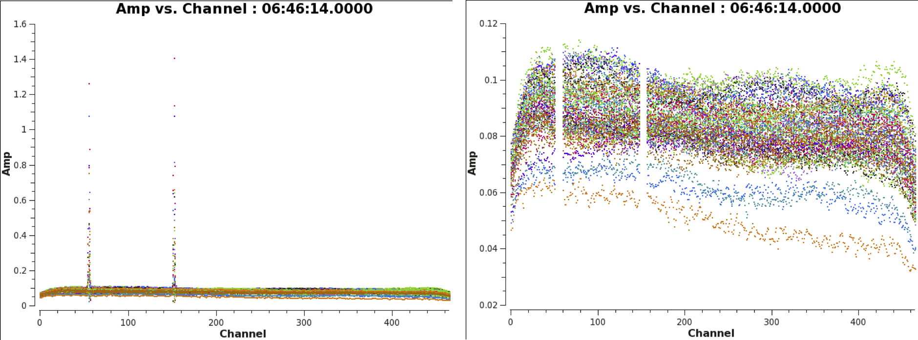
We will now perform a more in-depth flagging of the bad data. Our strategy is to first focus on the calibrator source (in this case only 3C48). If the calibrator data are flagged well, we should be able to perform an accurate calibration of the target data. Later in this document we will then flag the calibrated target data using an automated flagger.
When plotting amplitude vs frequency in CASA task plotms, we see that there are still two ranges of channels filled with RFI throughout the observing run (see Figure 2).
# In CASA
plotms(vis='MG0414_d1_data.ms',antenna='ea01',xaxis='chan',yaxis='amp',correlation='xx,yy',coloraxis='baseline', scan='7',averagedata=True, avgtime='1e9')
We will flag this data with the CASA task flagdata. Because we are flagging channels on all scans of the bandpass calibrator 3C48, these channels cannot be calibrated accurately, so we flag these channels also in the data of the target.
# In CASA
flagdata(vis='MG0414_d1_data.ms', mode='manual', spw='0:148~155', action='apply')
flagdata(vis='MG0414_d1_data.ms', mode='manual', spw='0:51~59', action='apply')
The data on our bandpass+gain+flux calibrator 3C48 now look clean, with no dead or misbehaving antennas. We can repeat the same plotms call as above:
# In CASA
plotms(vis='MG0414_d1_data.ms',antenna='ea01',xaxis='chan',yaxis='amp',correlation='xx,yy',coloraxis='baseline', scan='7',averagedata=True, avgtime='1e9')
We now start with the calibration.
Calibration
Many of the steps below are based on the CASA tutorial on reducing VLA P-band continuum data.
A priori Antenna Position Corrections
We start the calibration by obtaining the latest set of antenna-position corrections compared to the stored values that were derived at the start of the observing period. For this you need to run CASA task gencal with parameter caltype='antpos'. (Be sure to have internet connection in order to grab the antenna position corrections.)
# In CASA
gencal(vis='MG0414_d1_data.ms', caltype='antpos', caltable='antpos.cal')
The output is a list of antenna position corrections that are written to the calibration table antpos.cal:
2017-07-25 19:54:51 INFO gencal	 Determine antenna position offests from the baseline correction database
2017-07-25 19:54:52 INFO gencal	offsets for antenna ea01 :  0.00200   0.00000   0.00200
2017-07-25 19:54:52 INFO gencal	offsets for antenna ea02 :  0.00210   0.01800   0.00430
2017-07-25 19:54:52 INFO gencal	offsets for antenna ea03 : -0.00700   0.01600  -0.02000
2017-07-25 19:54:52 INFO gencal	offsets for antenna ea06 :  0.00200  -0.00200   0.00500
2017-07-25 19:54:52 INFO gencal	offsets for antenna ea08 : -0.01290   0.01280   0.02920
2017-07-25 19:54:52 INFO gencal	offsets for antenna ea09 : -0.01200  -0.01300   0.02400
2017-07-25 19:54:52 INFO gencal	offsets for antenna ea15 : -0.00500  -0.01000   0.01100
2017-07-25 19:54:52 INFO gencal	offsets for antenna ea16 :  0.01100  -0.01500  -0.01200
2017-07-25 19:54:52 INFO gencal	offsets for antenna ea17 : -0.01300   0.00000   0.05000
2017-07-25 19:54:52 INFO gencal	offsets for antenna ea18 : -0.00600   0.02200  -0.02000
2017-07-25 19:54:52 INFO gencal	offsets for antenna ea22 :  0.00600   0.00000   0.00000
2017-07-25 19:54:52 INFO gencal	offsets for antenna ea25 : -0.00140   0.00140  -0.00140
2017-07-25 19:54:52 INFO gencal	offsets for antenna ea27 : -0.00400  -0.00500   0.03100
2017-07-25 19:54:52 INFO gencal	offsets for antenna ea28 : -0.02100  -0.02900   0.01900
2017-07-25 19:54:52 INFO calibrater	Beginning specifycal-----------------------
2017-07-25 19:54:52 INFO  	Creating KAntPos Jones table from specified parameters.
2017-07-25 19:54:52 WARN  	NB: This EVLA dataset appears to fall within the period
2017-07-25 19:54:52 WARN +	  of semester 16B during which the online tropospheric
2017-07-25 19:54:52 WARN +	  delay model was mis-applied.
2017-07-25 19:54:52 WARN  	A correction for the online tropospheric delay model error WILL BE APPLIED!
2017-07-25 19:54:52 WARN  	Marking antpos caltable to turn ON the trop delay correction.
Note that these observations were taken during a period in which the atmospheric delay terms were calculated incorrectly. In CASA versions 4.7.1 and up a correction for this term is taken into account automatically when running CASA task gencal with parameter caltype='antpos'.
Ionospheric calibration
At frequencies below 5 GHz, ionospheric effects may need to be corrected. These corrections become important for frequencies < 1 GHz. CASA’s strategy is to obtain information on the total electron content (TEC) for the date of observations, which is based on data from the global navigation satellite system (GNSS). A series of CASA images in the form of a 24 hour movie of the TEC, as function of longitude and latitude, is then generated and stored as filename.IGS_TEC.im, with a corresponding TEC error movie named filename.IGS_RMS_TEC.im (these movies can be viewed in CASA’s viewer (please note that this task is deprecated, and in the future CARTA should be used for the visualizations). In order to download the data, you need to be connected to the internet:
# In CASA

from casatasks.private import tec_maps

tec_image, tec_rms_image, plotname = tec_maps.create(vis='MG0414_d1_data.ms', doplot=True)
If, for any reason, the file cannot be retrieved from the server automatically, you can also download this specific TEC file for the tutorial here.
The information regarding the TEC is sparse and either active or direction-dependent ionospheric conditions may not be corrected very well. Also, the online TEC information improves with time, hence the quality of these data is best about two weeks after the observations.
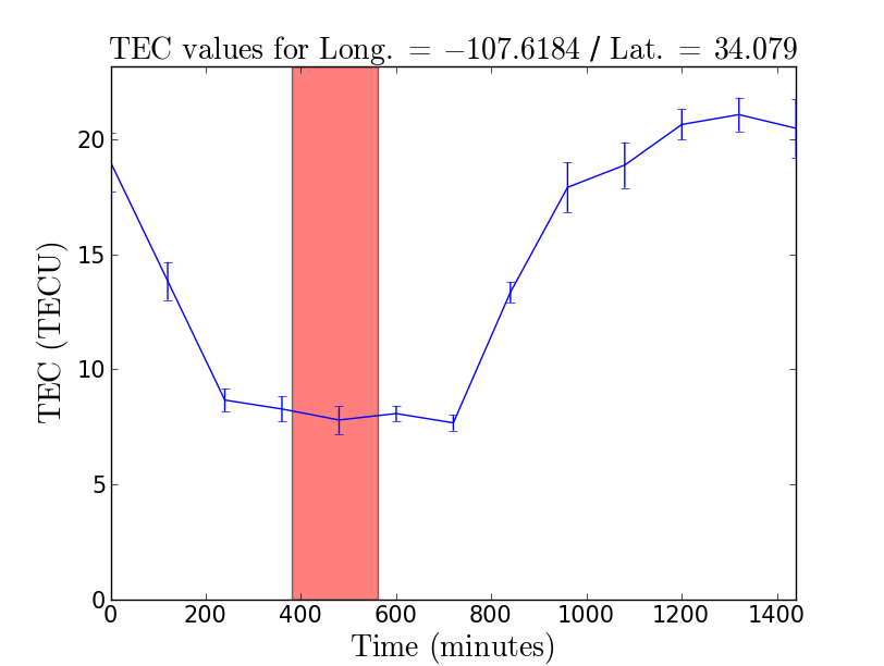
An ionosphere correction table is subsequently generated using CASA task gencal, in which the projected line-of-sight TEC (which depends on the zenith angle) is sampled for all times in the observation and stored in a standard CASA caltable. Figure 3 shows a plot that is generated for this caltable and can be opened using xv.
# In CASA
gencal(vis='MG0414_d1_data.ms', caltype='tecim', caltable='tecim.cal',infile=tec_image)
See the CASA Cookbook 4.7.2 for a detailed description on ionosphere corrections in CASA (thanks are due to Jason Kooi, University of Iowa, for his contributions).
Calibration of requantizer gains
Next we will calibrate the requantizer gain levels, which are the visibility amplitudes that were set as the input of the WIDAR correlator. Requantizer scans are added to a P-band observation to optimize the digital power in each spectral window which, in turn, maximizes the signal-to-noise of each window. Because there is a significant variation in power across the 240 MHz of P-band, and because some spectral windows may experience a high power due to strong RFI, setting the requantizer levels during the observations may improve the quality of the data, including the shape of the bandpass across multiple spectral windows. As part of the test observations of MG0414+0534, the very strong source Cygnus A was observed at the start of the run. Re-setting the requantizer levels both before observing Cygnus A and before targeting the other (much weaker) sources was essential to optimize the digital power and avoid correlation errors. Although we do not use Cygnus A as part of this tutorial, and we use only a single spectral window, performing calibration of the requantizer gains is still good practice for P-band spectral line reduction using CASA task gencal.
# In CASA
gencal(vis='MG0414_d1_data.ms', caltype='rq', caltable='rq.cal')
Initial absolute flux density scale calibration
The next step is to set the absolute flux levels of our flux calibrator 3C48 (field='0' from our listobs output), for which a well-known model exists using CASA task setjy:
# In CASA
setjy(vis='MG0414_d1_data.ms', field='0', scalebychan=True, standard='Perley-Butler 2017', listmodels=False, usescratch=True)
It is crucial for spectral line work to set the parameter scalebychan=True to ensure that the absolute flux level is calculated per channel and correctly interpolated across the observing band. If scalebychan=False, then only a single value per spectral window is calculated, resulting in a step function in flux between spectral windows.
Delay calibration
The delay of each antenna, for each polarization and each spectral window, is now determined. Doing this on a short scan of the primary calibrator is generally sufficient and will correct for both internal (e.g., electronics, cables) and external (e.g., ionosphere) effects. We select ea04 as reference antenna as it produced good data, has baselines to all other used antennas in the array, and is located in the center of the array. We also need to apply, "on-the-fly," the calibration tables for the antenna positions, the total electron content, and the requantizer levels using the CASA task gaincal.
# In CASA
gaincal(vis='MG0414_d1_data.ms', caltable='delays.cal', field='0', selectdata=True, timerange='06:43:48~06:48:42', solint='inf', refant='ea04', gaintype='K', gaintable=['antpos.cal','tecim.cal','rq.cal'])
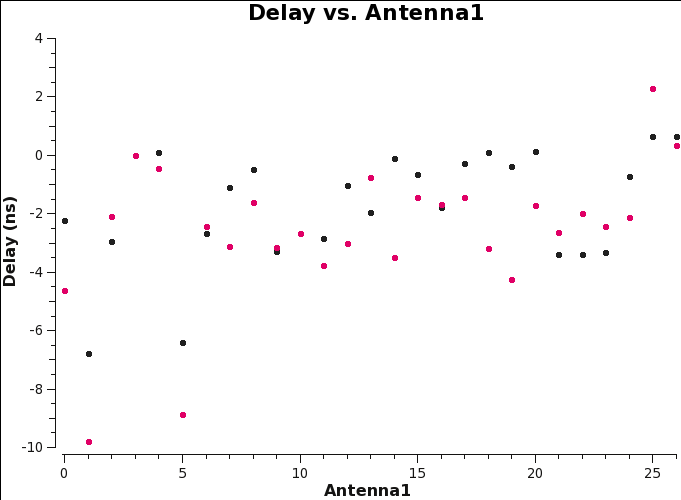
The calibration solutions can be plotted using CASA task plotms (see Figure 4):
# In CASA
plotms(vis='delays.cal',xaxis='antenna1',yaxis='delay',field='0',coloraxis='corr')
Note that any delays deviating by more than 30 nsec should be treated with caution and, if needed, flagged.
Bandpass calibration
Next step is to calibrate the bandpass, which corrects for the frequency dependent gain variations. Before determining the frequency dependent gains, we first calibrate the phases in time, deriving a solution for each integration, to make sure that we can derive accurate bandpass solutions when integrating over a full scan on the bandpass calibrator 3C48. This is done using CASA task gaincal:
# In CASA
gaincal(vis='MG0414_d1_data.ms', caltable='bpphase.gcal', field='0', spw='0:250~300', refant='ea04', calmode='p', solint='int', minsnr=3.0, gaintype='G', gaintable=['antpos.cal','tecim.cal','rq.cal','delays.cal'])
We use these phase solutions to perform the actual bandpass calibration. In this case, we have scans of our bandpass calibrator 3C48 taken at three different times during the observation. By interpolating the bandpass solutions in time, we try to minimize any possible time-varying bandpass effects and improve our spectral dynamic range. Bandpass calibration is performed in CASA by the task bandpass:
# In CASA
bandpass(vis='MG0414_d1_data.ms', caltable='bandpass.cal', field='0', spw='0', solint='inf', combine='', refant='ea04', solnorm=False, bandtype='B', gaintable=['antpos.cal','tecim.cal','rq.cal','delays.cal','bpphase.gcal'])
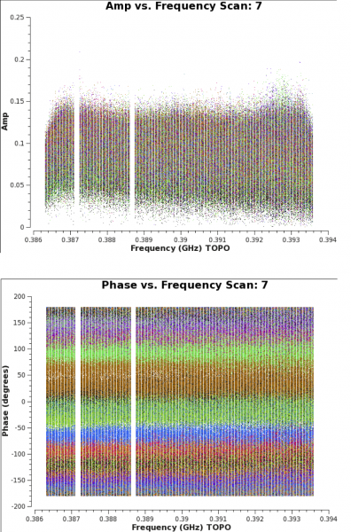
To interpolate between bandpass scans, it is essential to specify parameter combine=' '. The reason being that the default of combine='scan', when coupled with the parameter solint='inf', would cross the scan boundaries to form one single solution for the bandpass. Only when combining solint='inf' with combine=' ' is a bandpass solution obtained for each individual scan on 3C48. The bandpass plots can be viewed using CASA task plotms (see Figure 5).
# In CASA
plotms(vis='MG0414_d1_data.ms',field='0',antenna='ea04', xaxis='frequency',yaxis='amp',scan='7',correlation='xx,yy', coloraxis='baseline')
plotms(vis='MG0414_d1_data.ms',field='0',antenna='ea04', xaxis='frequency',yaxis='phase',scan='7',correlation='xx,yy', coloraxis='baseline')
Gain calibration
After the bandpass calibration, we perform a phase calibration of our data. Because we apply the bandpass solutions "on-the-fly," we can use the full bandwidth to determine the phase solutions. We will create two different calibration tables to correct for the time-varying phases. First we calibrate the phases on each interval with the CASA task gaincal parameter of solint set to int:
# In CASA
gaincal(vis='MG0414_d1_data.ms', caltable='intphase.gcal', field='0', spw='0', refant='ea04', calmode='p', solint='int', minsnr=3.0, gaintable=['antpos.cal','tecim.cal','rq.cal','delays.cal','bandpass.cal'])
The sole purpose of generating phase solutions on each 10 second interval is to be able to accurately correct for the time-varying amplitudes as we will see below. This method, however, is not ideal for interpolating the phase solutions in time. For that we do a second phase calibration, this time averaging the signal across the phase calibrator scans with the CASA task gaincal parameter of solint='inf':
# In CASA
gaincal(vis='MG0414_d1_data.ms', caltable='scanphase.gcal', field='0', spw='0', refant='ea04', calmode='p', solint='inf', combine='', minsnr=3.0, gaintable=['antpos.cal','tecim.cal','rq.cal','delays.cal','bandpass.cal'])
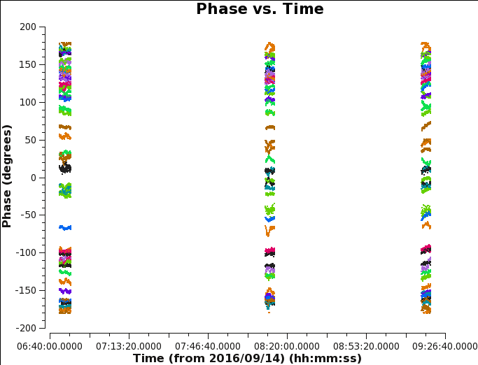
Note that an alternative approach to deriving phase solutions per scan is to use the CASA task smoothcal to average the phase corrections obtained every 10s with solin='int' over the full duration of a single scan. Generate a phase plot using CASA task plotms with the parameters below (see Figure 6):
# In CASA
plotms(vis='MG0414_d1_data.ms',field='0',antenna='ea04', correlation='xx,yy',avgchannel='1e8', xaxis='time',yaxis='phase',coloraxis='baseline')
We have selected an arbitrarily high number for the average channel to ensure it will include all of them. It will led to a warning message on the terminal screen.
Scaling the Amplitude Gains
We now perform a calibration of the amplitude variations in time. For this, we will apply the phase solution obtained in each 10 second interval via CASA task gaincal:
# In CASA
gaincal(vis='MG0414_d1_data.ms', caltable='amp.gcal', field='0', spw='0', selectdata=False, solint='inf', combine='', refant='ea04', calmode='ap', minsnr=3.0, gaintable=['antpos.cal','tecim.cal','rq.cal','delays.cal','bandpass.cal','intphase.gcal'])
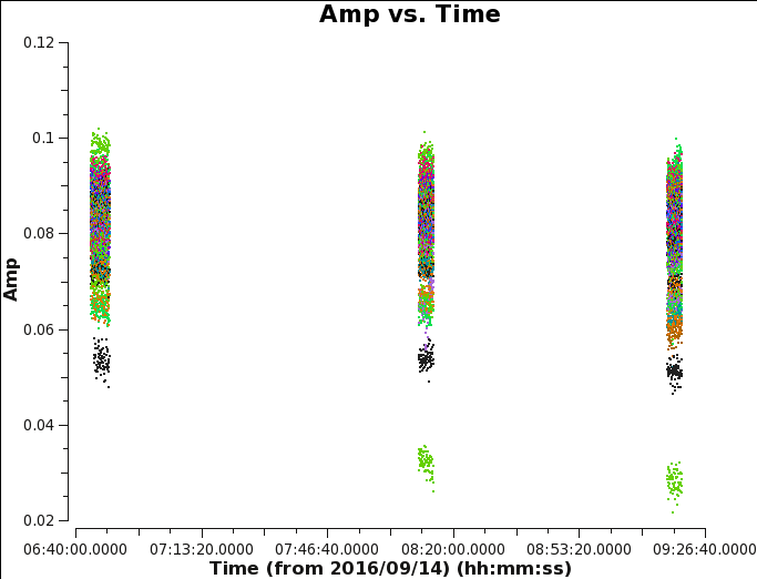
Normally this procedure will only calibrate the relative amplitudes, and the CASA task fluxscale is required to place the data on an absolute flux density scale. However, because our flux-calibrator is also our bandpass and gain calibrator, the absolute flux density scale will already be ok, so we can skip this step. Generate an amplitude gain plot using CASA task plotms (see Figure 7) with the parameters below:
# In CASA
plotms(vis='MG0414_d1_data.ms',field='0',antenna='ea04', correlation='xx,yy',avgchannel='1e8', xaxis='time',yaxis='amp',coloraxis='baseline')
Applying the calibration
We have now finished the calibration of the data. We will apply the calibration tables that were derived from 3C48 to both the calibrator 3C48 itself and our target MG0414+0354. The CASA task applycal creates a corrected data column where the calibrated data are stored.
# In CASA
applycal(vis='MG0414_d1_data.ms', field='0', gaintable=['antpos.cal','tecim.cal','rq.cal','delays.cal','bandpass.cal','scanphase.gcal','amp.gcal'], gainfield=['','','','0','0','0','0'], parang=True, calwt=False, applymode='calflagstrict', flagbackup=True)
# In CASA
applycal(vis='MG0414_d1_data.ms', field='1', gaintable=['antpos.cal','tecim.cal','rq.cal','delays.cal','bandpass.cal','scanphase.gcal','amp.gcal'], gainfield=['','','','0','0','0','0'], calwt=False, applymode='calflagstrict', flagbackup=True)
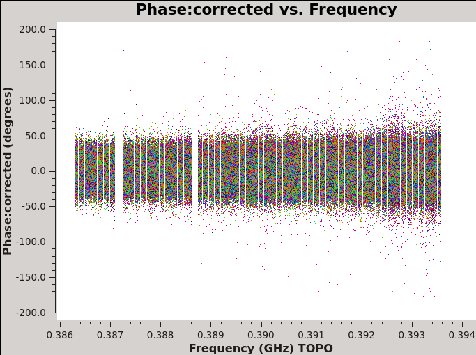
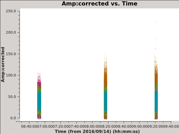
Sometimes after calibrating the data it is easier to see any offending antennas or baselines. Replotting with ydatacolumn='corrected' will produce the corrected calibration plots (Figures 8a-d).
# In CASA for corrected amplitude and phase vs frequency, Figures 8a and 8b
plotms(vis='MG0414_d1_data.ms',field='0',antenna='ea04', xaxis='frequency',yaxis='amp',scan='7',ydatacolumn='corrected',correlation='xx,yy', coloraxis='baseline')
plotms(vis='MG0414_d1_data.ms',field='0',antenna='ea04', xaxis='frequency',yaxis='phase',scan='7',ydatacolumn='corrected',correlation='xx,yy', coloraxis='baseline')
# In CASA for corrected amplitude and phase vs time, Figures 8c and 8d
plotms(vis='MG0414_d1_data.ms',field='0',antenna='ea04', correlation='xx,yy', xaxis='time',yaxis='amp',ydatacolumn='corrected',coloraxis='baseline')
plotms(vis='MG0414_d1_data.ms',field='0',antenna='ea04', correlation='xx,yy',avgchannel='1e8', xaxis='time',yaxis='phase',ydatacolumn='corrected',coloraxis='baseline')
The calibrated data of the primary calibrator 3C48 show that the YY amplitudes of ea17 are off during the second part of the run (see the green points with low values in figure 7). Because calibration solutions are antenna based, to get the best calibration, flag any poor data and re-run the calibration process. A currently known issue is that CASA task gaincal will not find good solutions if any correlation, including cross-correlation, in the data is completely flagged. In this case, there is no difference between flagging only the YY polarization of ea17 or the entire antenna.
Antenna ea17 will be flagged using CASA task flagdata:
# In CASA
flagdata(vis='MG0414_d1_data.ms', mode='manual', antenna='ea17', action='apply')
 |
 |
 |
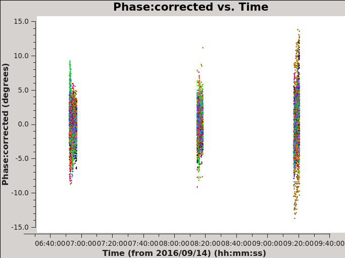 |
| Figure 8a. Effects of bandpass calibration on the frequency dependent amplitudes across the observing band. The plots were made in CASA task plotms and in the Axes tab choosing option Y Data Column: corrected. | Figure 8b. Effects of bandpass calibration on the frequency dependent phases across the observing band. The plots were made in CASA task plotms and in the Axes tab choosing option Y Data Column: corrected. | Figure 8c. Effects of phase calibration on the time dependent amplitudes across the observing band. The various colors show the different baselines with reference antenna ea04. The plot was made in CASA task plotms and in the Axes tab choosing option Y Data Column: corrected. | Figure 8d. Effects of phase calibration on the time dependent phases across the observing band. The various colors show the different baselines with reference antenna ea04. The plot was made in CASA task plotms and in the Axes tab choosing option Y Data Column: corrected. |
Then run the calibration process again starting with the Delay calibration:
# In CASA
gaincal(vis='MG0414_d1_data.ms', caltable='delays.cal', field='0', selectdata=True, timerange='06:43:48~06:48:42', solint='inf', refant='ea04', gaintype='K', gaintable=['antpos.cal','tecim.cal','rq.cal'])

gaincal(vis='MG0414_d1_data.ms', caltable='bpphase.gcal', field='0', spw='0:250~300', refant='ea04', calmode='p', solint='int', minsnr=3.0, gaintype='G', gaintable=['antpos.cal','tecim.cal','rq.cal','delays.cal'])

bandpass(vis='MG0414_d1_data.ms', caltable='bandpass.cal', field='0', spw='0', solint='inf', combine='', refant='ea04', solnorm=False, bandtype='B', gaintable=['antpos.cal','tecim.cal','rq.cal','delays.cal','bpphase.gcal'])

gaincal(vis='MG0414_d1_data.ms', caltable='intphase.gcal', field='0', spw='0', refant='ea04', calmode='p', solint='int', minsnr=3.0, gaintable=['antpos.cal','tecim.cal','rq.cal','delays.cal','bandpass.cal'])

gaincal(vis='MG0414_d1_data.ms', caltable='scanphase.gcal', field='0', spw='0', refant='ea04', calmode='p', solint='inf', combine='', minsnr=3.0, gaintable=['antpos.cal','tecim.cal','rq.cal','delays.cal','bandpass.cal'])

gaincal(vis='MG0414_d1_data.ms', caltable='amp.gcal', field='0', spw='0', selectdata=False, solint='inf', combine='', refant='ea04', calmode='ap', minsnr=3.0, gaintable=['antpos.cal','tecim.cal','rq.cal','delays.cal','bandpass.cal','intphase.gcal'])
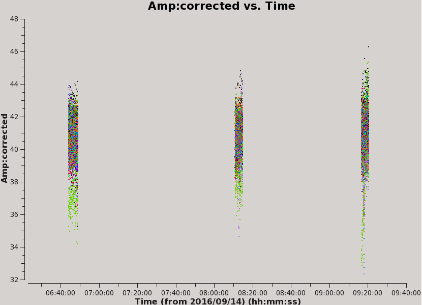
The new calibration tables have overwritten the previous tables. Once you've re-run the calibration, you need to apply it.
# In CASA
applycal(vis='MG0414_d1_data.ms', field='0', gaintable=['antpos.cal','tecim.cal','rq.cal','delays.cal','bandpass.cal','scanphase.gcal','amp.gcal'], gainfield=['','','','0','0','0','0'], parang=True, calwt=False, applymode='calflagstrict', flagbackup=True)

applycal(vis='MG0414_d1_data.ms', field='1', gaintable=['antpos.cal','tecim.cal','rq.cal','delays.cal','bandpass.cal','scanphase.gcal','amp.gcal'], gainfield=['','','','0','0','0','0'], calwt=False, applymode='calflagstrict', flagbackup=True)
And then, plot the corrected amplitudes vs time with ea17 flagged (see Figure 9):
# In CASA for corrected amp vs time with ea17 flagged, Figure 9
plotms(vis='MG0414_d1_data.ms',field='0',antenna='ea04', correlation='xx,yy',avgchannel='1e8', xaxis='time',yaxis='amp',ydatacolumn='corrected',coloraxis='baseline')
We now split the calibrated data of our target into a new measurement set, including only the XX and YY polarization products. Using CASA task split the calibrated target data are placed into the data column of the new measurement set:
# In CASA
split(vis='MG0414_d1_data.ms', outputvis='MG0414_d1_calibrated.ms', datacolumn='corrected', field='1', correlation='xx,yy', keepflags=False)
Imaging and Self-calibration
We now have a calibrated data set that has all calibration applied except for possible self-calibration. Self-calibration relies on the target itself to better calibrate antenna-based gains (phases and amplitudes) as a function of time. It can be applied to targets that are strong in the continuum or have a strong enough spectral line to derive good phase and, if desired, also amplitude solutions on short (order of minutes) timescales. The procedure relies on an initial model of the target, which then can be used iteratively to improve the gains and hence the quality of the image itself. Here we show the various steps in self-calibrating our data based on the strong continuum emission of MG0414+0354. Please refer to a dedicated CASA guide on self-calibration for further details.
If strong RFI is present in the target, it may be necessary to flag your data before proceeding with self-calibration. This is not the case with MG0414+0354.
We create an initial model of our target field using CASA task tclean. Notice that we will exclude from the continuum image the channels that we have flagged and the channels where we expected to detect the line:
# In CASA
tclean(vis='MG0414_d1_calibrated.ms', datacolumn='data', imagename='MG0414_d1_cont_R03', spw='0:4~50;60~147;156~250;350~460', specmode='mfs', niter=100, threshold='1.5Jy', imsize=[256,256], cell='1arcsec', weighting='briggs', robust=0.2, savemodel='modelcolumn')
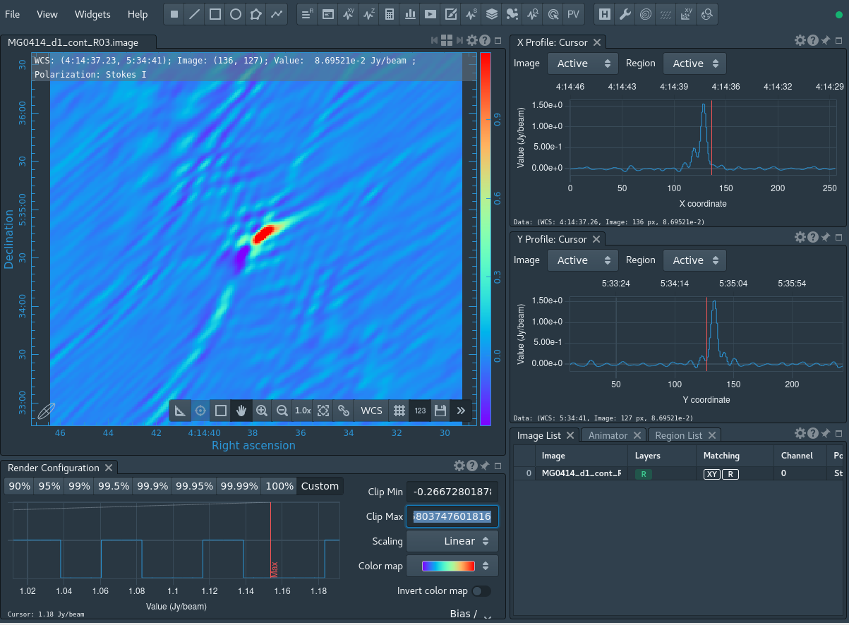
The information in the MODEL column consist of visibilities that present a model of the target field. CASA task tclean produces a .model image of the model that you can visualize with CARTA software. It is essential that only components that you know for sure represent the continuum in the target field are taken into account in self-calibration. If this is not the case, you probably cleaned too deep and included noise features or artifacts (e.g., from the beam-pattern) in the model. Self-calibration would permanently lock these as features in your data, so this should be avoided. On the other hand, it is equally crucial to ensure that the model is not empty, as this will result in your target being shifted to the phase center.
You can see the tclean results using the CARTA tool, as we show in figure 10. Please refer to the CASA documentation on how to load the image into CARTA.
Next, we derive phase corrections to this model. Because our target is strong enough to do self-calibration on it, we should get enough S/N per baseline on a 60 sec interval, using CASA task gaincal:
# In CASA
gaincal(vis='MG0414_d1_calibrated.ms', caltable='sc1.gcal', field='0', spw='0', refant='ea04', calmode='p', solint='60s', combine='', minsnr=3.0)
This creates a new phase-calibration table that we call sc1.gcal. We now apply this calibration table to the calibrated data in order to improve the phase-only solutions using CASA task applycal:
# In CASA
applycal(vis='MG0414_d1_calibrated.ms', field='0', gaintable=['sc1.gcal'], interp='linear')
Because self-calibration is an iterative process, we want to repeat this step again in order to further improve the gain calibration. For that, we first split the data calibrated with the self-calibration solutions applied to the DATA column to a new measurement set, again using CASA task split:
# In CASA
split(vis='MG0414_d1_calibrated.ms', outputvis='MG0414_d1_sc1.ms', datacolumn='corrected', field='0', keepflags=False)
Now we can use this newly created measurement set to make a better continuum image and subsequently perform the next round of self-calibration:
# In CASA
tclean(vis='MG0414_d1_sc1.ms', datacolumn='data', imagename='MG0414_d1_cont_sc1.R03', spw='0:4~50;60~147;156~250;350~460', specmode='mfs', niter=500, threshold='500mJy', imsize=[256,256],cell='1arcsec', weighting='briggs', robust=0.2, savemodel='modelcolumn')
# In CASA
gaincal(vis='MG0414_d1_sc1.ms', caltable='sc2.gcal', field='0', spw='0', refant='ea04', calmode='p', solint='30s', combine='', minsnr=3.0)
# In CASA
applycal(vis='MG0414_d1_sc1.ms', field='0', gaintable=['sc2.gcal'], interp='linear')
# In CASA
split(vis='MG0414_d1_sc1.ms', outputvis='MG0414_d1_sc2.ms', datacolumn='corrected', field='0', keepflags=False)
# In CASA
tclean(vis='MG0414_d1_sc2.ms', datacolumn='data', imagename='MG0414_d1_cont_sc2_R03', spw='0:4~50;60~147;156~250;350~460', specmode='mfs', niter=1000, threshold='100mJy', imsize=[256,256], cell='1arcsec', weighting='briggs', robust=0.2, savemodel='modelcolumn')
Now that we have a good model of the continuum in the field of MG0414+0354, we will attempt a final self-calibration using both the phases and amplitudes via CASA task gaincal :
# In CASA
gaincal(vis='MG0414_d1_sc2.ms', caltable='sc3ap.gcal', field='0', spw='0', refant='ea04', calmode='ap', solint='30s', combine='', minsnr=3.0, solnorm=True)
# In CASA
applycal(vis='MG0414_d1_sc2.ms', field='0', gaintable=['sc3ap.gcal'], interp='linear')
# In CASA
split(vis='MG0414_d1_sc2.ms', outputvis='MG0414_d1_sc3ap.ms', datacolumn='corrected', field='0', keepflags=False)
# In CASA
tclean(vis='MG0414_d1_sc3ap.ms', datacolumn='data', imagename='MG0414_d1_cont_sc3ap_R03', spw='0:4~50;60~147;156~250;350~460', specmode='mfs', niter=1000, threshold='100mJy', imsize=[256,256], cell='1arcsec', weighting='briggs', robust=0.2, savemodel='modelcolumn')
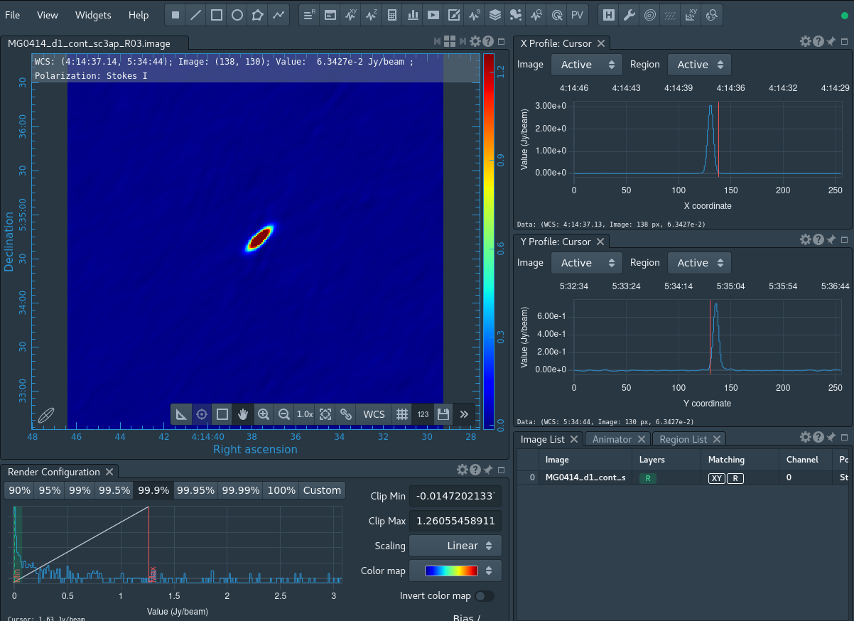
The output continuum image from the last iteration of CASA task tclean continues to be an improvement over previous imaging, as you can see using CARTA again (Figure 11 showing results after three passes of self-calibration).
However, now it also shows that we are not likely to gain further improvement with additional rounds of self-calibration (you can inspect this yourself by comparing the images created across the different iterations in CARTA). This indicates that we now have a calibrated data-set of MG0414+0354 that is almost ready for final imaging. Before imaging, we need to flag the target data to remove poor-quality data. First, we run an automated flagging routine using CASA task flagdata with the parameter mode='rflag':
# In CASA
flagdata(vis='MG0414_d1_sc3ap.ms', mode='rflag', datacolumn='data')
After having ran this automated flagging, we inspect the data via the CASA task msview by displaying time vs channel for the different baselines, or you may display time vs baseline for the different channels:
# In CASA
msview('MG0414_d1_sc3ap.ms')
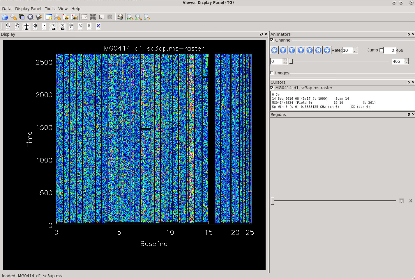
Keep in mind that when the data is properly calibrated, it is easier to recognize low-level imperfections which may have to be flagged to improve the image quality. In this case, the noisier baselines are seen with lighter colors (see Figure 12). Hovering over these baselines will report a number pair such as 8-16, 8-17, etc. in the msview. From this we can tell that baselines 8-# and 12-# (which correspond to antennas ea09 and ea14) have significantly higher noise than the other antennas, something which was not picked up by the automated flagging routine. Additionally, for a number of baselines, the data quality looks relatively poor. We flag these antennas and baselines via the CASA flagdata task before imaging the data.
# In CASA
flagdata(vis='MG0414_d1_sc3ap.ms', mode='manual', antenna='ea09', datacolumn='data')
flagdata(vis='MG0414_d1_sc3ap.ms', mode='manual', antenna='ea14', datacolumn='data')
To flag offending individual baselines, in CASA task flagdata you may use antenna='antenna&antenna(&antenna...)'.
Flagging data can be an iterative process. Often, the better the data is calibrated, the easier it is to recognize low-level imperfections in it. To optimize the data reduction, you can script the calibration process, and opt to flag the data also in the original data set (i.e., before calibration), after which you run the entire calibration again.
When you flag these antennas on the MS before the self calibration took place, you must go back and rerun the calibration before the final imaging, starting at the Delay calibration section. If you rerun the calibration you will either have to rename your measurement sets created from split during self calibration, or delete them in order to redo self calibration as split will not overwrite a ms name.
We image the data using the CASA task tclean. A 0.5Jy threshold was chosen for this command by interactively cleaning a single channel of the final self calibrated image and taking the 5σ of the noise levels once the image was cleaned. With an ideal threshold found, we can now clean all channels (this process can take hours to complete depending on the machine you are using):
# In CASA
tclean(vis='MG0414_d1_sc3ap.ms', datacolumn='data', imagename='MG0414_d1_line_sc3ap_vel_R03', spw='0', specmode='cube', outframe='bary', veltype='optical', restfreq='390.600MHz', niter=10000000, threshold='0.05Jy', imsize=[256,256], cell='1arcsec', pbcor=True, weighting='briggs', robust=0.2, perchanweightdensity=True, savemodel='none',interpolation='nearest')
OBS: From CASA version 6.2.0 onwards, one new input parameter has been added to the task tclean. The psfcutoff parameter allows fitting non-Gaussian PSF. The default value is 0.35, but can vary from 0.01 to 0.99. It is a parameter for advanced users, and it should rarely be changed. If a user needs to use it, the resulting fits should be carefully checked. We have used the default value in all tclean runs of this tutorial since we have not set it at any time.
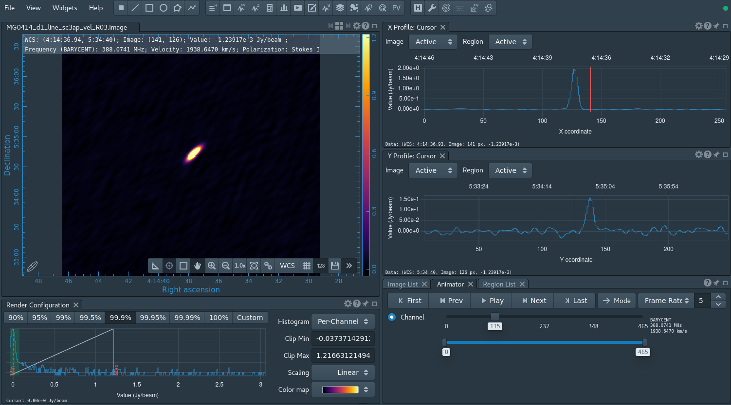
We can inspect the resulting line-data cube, again using CARTA. The HI absorption feature is clearly present (see Figure 14). If you did NOT re-run the calibration sequence, you should get a plot that should look similar to Figures 13 and 14. To see your spectral line, open the last image of the source. Go to a channel that shows the source, then zoom in on the source. Click the Point marking icon, find the brightest pixel in the source and click on it. Now click on the spectral profile tool button to get the single point profile of the spectrum. Here you will see a spectrum with 2 dips that drop to zero; these dips are a part of the flagging we have done. You will need to zoom in in order to notice any spectral lines due to the auto scaling; zoom in by clicking on the graph and creating a yellow box then release.
The data cube contains both continuum and line emission, which can optionally be separated using the CASA task uvcontsub. In principle, this task can be used for continuum subtraction and fitting in the uv domain; however, combining spws for the continuum fitting is not yet supported in the updated uvcontsub in CASA 6.5.2, and for that particular functionality the uvcontsub_old should be used for the time being.
Last checked on CASA Version 6.5.2