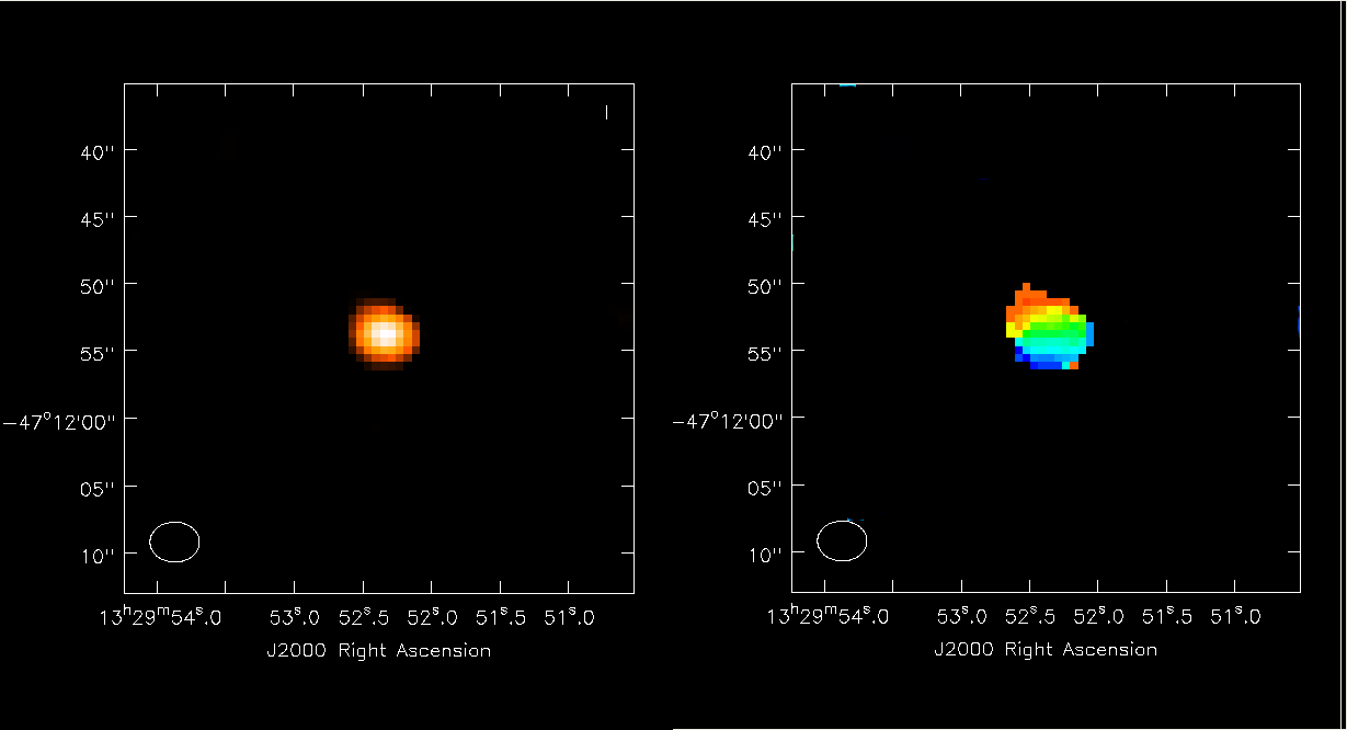
M51 at z = 0.1 and z = 0.3 (CASA 3.1)
↵ Simulating Observations in CASA 3.1
Remember that you need to follow this process: Extracting scripts from these tutorials to extract a casapy script from this web page.
Overview
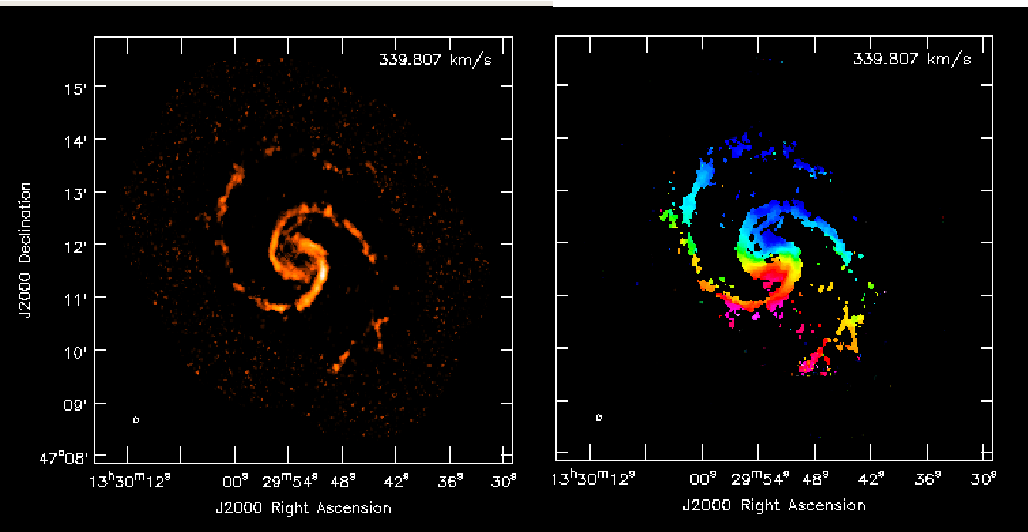
This tutorial presents a simulation of ALMA observations of the well-known galaxy M51 in the CO 1-0 transition. This galaxy is located relatively nearby (luminosity distance = 9 Mpc), but, in this simulation, we will model how it would appear at redshift z = 0.1 (luminosity distance = 460 Mpc).
The goal of this tutorial is to provide a complete run-through of a relatively simple simulation. Included in this simulation are the effects of (u, v) sampling of a 50-antenna ALMA, the primary beam of the ALMA, and thermal noise. Neither calibration overheads nor errors are included, and so this simulation should be viewed as optimistic.
For this tutorial, we'll use the BIMA SONG (Helfer et al. 2003) observations of M51 as the basis for the model. Grab the file NGC5194.bima12m.cm.fits.gz and uncompress it in a working directory.
# in bash (or other unix shell)
gunzip NGC5194.bima.12m.cm.fits.gz
Load these data into CASA. For convenience, store the name of the resulting measurement set into the python global cubeName.
cubeName = 'm51-song'
importfits(fitsimage='NGC5194.bima12m.cm.fits', imagename=cubeName)
# initialize simdata
default("simdata")
skymodel=cubeName
modifymodel=True
Noise in the Input Model
The input model is actually an observation and, as such, certainly contains noise. We're OK as long as the noise in the model falls below the expected thermal noise of the ALMA observation. Here's a quick, back-of-the-envelope calculation.
The noise on the BIMA SONG channels measures roughly 0.1 Jy/beam, which scales to 0.04 mJy/beam at z = 0.1 (to within factors of powers of 1+z for cosmology and root-small-integer for the to-be-degraded beam; see below). For comparison, the expected thermal noise of the ALMA observation is 0.1 mJy / beam (using the ALMA Sensitivity Calculator, assuming 8 hrs integration, and, to match roughly the BIMA SONG observation, a 4 MHz channel width), a factor of 2.5 greater than the anticipated contribution of noise from the model. Added in quadrature, the noise components total 0.108 mJy, and so we can expect that the input model noise degrades the simulation noise by about 8%.
Cosmology Calculations
Next we'll set up some python globals to handle the scaling of the model coordinates and flux densities appropriate for new redshift. We'll primarily need the angular size and luminosity distances for a given cosmology. To keep things simple, we'll use Ned Wright's CosmoCalc (2006) with the default cosmology; redshifts were collected from NED.
#z's
# Distinguish between z_lsrk, which sets the observed frequency for scaling, from z_cmb,
#      which is needed to get cosmological distances.
z_old_cmb = 0.002122 # CMB-referenced z for cosmological distances from NED
z_old_lsrk = 0.001544 # from NED
z_new = 0.1
#
# angular size distances from CosmoCalc
da_old = 9.0
da_new = 375.9
#
# luminosity distances from CosmoCalc
dl_old = 8.937
dl_new = 454.8
The convention is old refers to M51 as observed at its proper redshift, and new refers to the new, higher redshift for our model.
Preparing the Model
The next step is to scale the M51 data cube into a model cube appropriate for simdata. First, we'll set up some globals to establish some file naming conventions.
suffix = "-p1" # z = 0.1, or point-1; useful to distinguish from repeated simulations at different z's
project = "M51-ATZ" + suffix  # project ID to assign output filenames (simdata parameter)
Flux Density Scaling
Our goal in this step is to set the inbright parameter of simdata, which will scale the data cube appropriately for its new luminosity distance.
Simdata wants models in units of Jy / pixel, but the BIMA SONG cube is in units of Jy / beam. That's an easy conversion.
# BIMA SONG beam
bmaj = imhead(imagename=cubeName,mode='get',hdkey='beammajor')
bmin = imhead(imagename=cubeName,mode='get',hdkey='beamminor')
#
# use qa tool to convert beam in radians to (1 arcsec) pixels:
bmaj = qa.convert(bmaj,'arcsec')['value']
bmin = qa.convert(bmin,'arcsec')['value']
#
toJyPerPix = 1.0 / (1.1331 * bmaj * bmin) # gaussian beam conversion = beams / pixel
Next, scale the flux for the new luminosity distance. Make the approximation that each pixel is a point source, and use the inverse square law to scale. Simdata can scale the peak surface brightness using the parameter inbright.
# correct flux density for luminosity distance
fluxScale = (dl_old/dl_new)**2 * (1.0 + z_new) / (1.0 + z_old_cmb)
# current peak flux:
peak = imstat(cubeName)['max'][0] * toJyPerPix # need to convert to Jy / pixel
# desired peak flux in Jy / pixel:
inbright = "%fJy/pixel" % (peak*fluxScale) # use python formatting convention
# inbright is a simdata parameter
Notice that there is an additional (1+z) correction because we are scaling flux densities rather than bolometric fluxes.
Angular Size Scaling
The sky coordinates axes of the model need to be adjusted (1) to place M51 in the southern hemisphere and (2) to correct for the new angular size distance. These tasks can be accomplished by the simdata parameters indirection (change the location of M51 on the sky) and incell (change the angular scale of an input pixel). a To perform task (1), we'll just flip the sign of the declination using imhead. Notice the use of the qa tool to convert radians to sexagesimal.
# Move to southern hemisphere.
# Use qa.formxxx tool to convert rad to sexagesimal.
# For clarity, build up "indirection" string one term at a time.
# Epoch
indirection = "J2000 " # parameter for simdata
# RA
indirection += qa.formxxx(imhead(imagename=cubeName,mode='get',hdkey='crval1')['value']+'rad',format='hms') + " "
# Dec * -1
indirection += qa.formxxx('%frad' % (-1*float(imhead(imagename=cubeName,mode='get',hdkey='crval2')['value'])),format='dms')
Next, adjust the pixel scale for the new angular size distance. To perform this adjustment, we'll use imhead with mode = "get" to read in the original pixel scale, and mode="put" to store the new pixel scale in the model header.
# scale pixel size:  imhead returns things in rad, so convert to arcsec
oldCell = float(imhead(imagename=cubeName,mode='get',hdkey='cdelt2')['value']) * 206265
# scale for new angular size distance
newCell = oldCell * da_old / da_new
# Format the new pixel size for input to simdata
incell = "%farcsec" % (newCell) # parameter for simdata
Adjusting the Frequency Axis
Changing the frequency axis of the model header is just a straightforward (1+z) correction. Simdata adjusts the channelwidth using the inwidth parameter and the observing frequency using incenter.
Notice that the absolute value of the BIMA SONG channel width is used. The noise calculation in Simdata needs positive channel widths, but the input cube is ordered in increasing velocity rather than increasing frequency. We could transpose the cube; on the other hand, the only penalty of changing the sign is that the sense of rotation will be flipped. Since this simulation is a simple detection experiment, the rotation sense is irrelevant, and so we'll take the easy way out.
# move freq to z_new
oldFreq = float(imhead(imagename=cubeName,mode='get',hdkey='crval3')['value'])   # Hz
newFreq = oldFreq * (1.0 + z_old_lsrk) / (1.0 + z_new)
nchan = imstat("NGC5194.bima12m.cm.fits")['trc'][2]
#
# Adjust frequency channelwidth for new z
oldDnu = float(imhead(imagename=cubeName,mode='get',hdkey='cdelt3')['value'])   # Hz
newDnu = abs((1.0+z_old_lsrk) /(1.0+z_new)*oldDnu) # need positive channel widths to ensure noise calc goes well
inwidth = "%fHz" % newDnu # parameter for simdata
#
# Specify the observing frequency at the center of the observing band:
incenter = "%fHz" % (newFreq + 0.5*nchan*newDnu)
Simdata
The CASA task simdata will monolithically simulate an ALMA observation, produce measurement sets with and without thermal noise, and finally produce a CLEANed image cube based on the simulated observation. Details can be found in the Simulating Observations in CASA tutorial.
The original BIMA SONG image is about 480 arcseconds across; scale this image size to the new redshift.
# estimate final image size
imSize = 480.0 * (da_old / da_new) # in arcseconds
For relatively high redshifts, there should be no need to mosaic the observations. We'll nevertheless allow for mosaicking in case we want to repeat the simulation for lower redshift. Simdata needs the spacing between pointings in the mosaic; we'll require pointings spaced by half of the primary beam.
# mosaicking info
primaryBeam = 17.0 * (300e9 / newFreq) # in arcseconds; ALMA primary beam = 17 arcsec at 300 GHz
pointingspacing = "%farcsec" % (primaryBeam / 2.0)
mapsize = "%farcsec" % imSize # how big to make the mosaic
We also need to estimate the desired synthesized beam size. We don't want the new beam to be so large so that we cannot resolve a rotation curve, but we also don't want it to be so small that we effectively resolve out the BIMA SONG data. The BIMA SONG beam was 5 arcsec, and so as a reasonable guess we'll adopt the equivalent of a 15" beam at its true distance(3 times coarser than the BIMA SONG beam) and then scale appropriately to z = 0.1.
# Estimate desired beam size. BIMA SONG has 5": use 15" projected to new redshift
beamNew = 15.0 * (da_old / da_new)
We want pixels that sample the beam at least 3 times for stable deconvolution; we'll use 4 times sampling, rounded off to the nearest milliarcsec.
pixelSize = round(beamNew * 1000.0 / 4.0) / 1000.0
Now, to guard against undersampling the beam as a result of rounding error, reset the desired beam to 4 times the pixel size.
beamNew = 4.0 * pixelSize
Now we know both the image size and pixel size in arcseconds, but simdata wants the ratio: the number of pixels along the RA or Dec axis. To keep the image from becoming too small, set the minimum image size to be 256 pixels.
imSizePix = int(round(imSize / pixelSize))
if imSizePix < 256: imSizePix = 256
Let simdata decide on an appropriate ALMA configuration based on the desired beam size. Set the parameter antennalist as follows (but see Other Antenna Configurations below).
predict=True
antennalist = "alma;%farcsec" % beamNew
Now we have enough information to run simdata, and hopefully some of the python global variables that were defined above will start to make sense. The following CASA and python commands set up the remaining parameters for the simdata task.
modelimage = cubeName
integration = '10s' # watch out for memory limits vs. ability to complete mosaic here
# 10s is usually safe for large mosaics, but will require more memory
totaltime = '28800s' # 8 hr integration
If you are doing this as a tutorial, we suggest that you consider increasing the integration time so that your learning is not slowed by processing time See Etime study for details.
# make simulated images/cubes
image=True
thermalnoise="tsys-atm" # add thermal noise, produce noisy.ms measurement set
vis = '$project.noisy.ms' # clean the data with *thermal noise added*
cell = "%farcsec" % pixelSize
imsize = [imSizePix,imSizePix]
threshold = "1.0mJy"
weighting = "natural"
stokes = 'I'
#
verbose = True
graphics="both"
overwrite = True
#
inp("simdata")
simdata()
Other Antenna Configurations
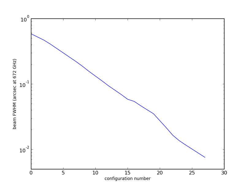
Finally, we need to know which ALMA configuration number based on the desired angular resolution. Simdata makes this easy by allowing users to specify the desired angular resolution in the parameter antennalist.
This tutorial is somewhat automated to produce a decent cube of M51 as viewed at z = 0.1. The selection of the ALMA antenna configuration is automated, but, for other simulations (or this one, for that matter), it will be worth playing with the configurations, or perhaps evaluating the possibility of detections in CSV or early science.
Notice from the simdata inputs that CASA comes with stock antenna configurations in the directory $CASAPATH/data/alma/simmos/ (the python task os.getenv is used to look up CASAPATH automatically). For CASA 3.0.1 and 3.1, here is a list of included antenna configurations.
| alma.csv.late.cfg |
| alma.csv.mid.cfg |
| alma.early.large.cfg |
| alma.early.med.cfg |
| alma.out01.cfg |
| alma.out02.cfg |
| alma.out03.cfg |
| ... |
| alma.out27.cfg |
| alma.out28.cfg |
There are also configuration data for the ACA, EVLA, and SMA.
Take a Break
If you have got this far, you've earned it. Simdata will be running for a while, and coffee sure sounds good right now.
Results
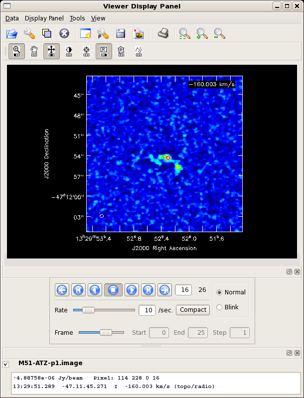
Here is an inventory of some of the simdata products.
| Filename | Description |
|---|---|
| M51-ATZ-p1.ms | Model measurement set sans noise |
| M51-ATZ-p1.noisy.ms | Model measurement set with thermal noise |
| M51-ATZ-p1.clean.image | CLEAN-deconvolved cube of M51-ATZ-p1.noisy.ms |
And there are plenty of other auxiliary files.
The rest frequency will have been lost in the simulation, and it's worth restoring to the header.
imhead(imagename="M51-ATZ-p1.image", mode="put", hdkey="restfreq", hdvalue="115.27120180GHz")
The simulated data cube can be analyzed just like any other CASA image -- examples are given in the CARMA tutorial and the VLA 21cm tutorial.
Moment Maps
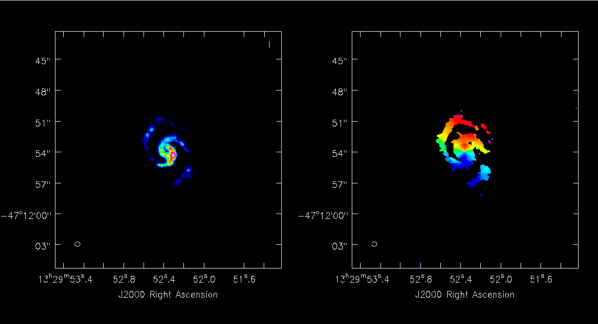
Use immoments to calculate the integrated intensity and velocity field maps from the simulated cube. The excludepix option applies a 3σ cut.
immoments(imagename='M51-ATZ-p1.image',moments=[0,1],axis='spectral',
          excludepix=[-100,0.0006],outfile='M51-ATZ-p1.moments')
The results are shown at right.
Pushing M51 out to z = 0.3
We'll leave it as an exercise how to tune this simulation to push M51 all the way out to z = 0.3 (luminosity distance = 1540 Mpc). Simdata produces a reasonable detection in 8 hrs integration, but you'll need to consider more carefully the antenna configuration needed to produce the requisite sensitivity. To conclude, here are the moment maps for the z = 0.3 simulation.
↵ Simulating Observations in CASA 3.1
Last checked on CASA Version 3.0.2 (r11631).
--Jack Gallimore 15:55, 30 April 2010 (UTC), updated for CASA 3.1 M. Lacy 1st December 2010
