Fit a Gaussian to Visibility data and plot it over the data
- DRAFT*
B.Mason, K.Ward-Duong, & J.Patience July 2015 developed in CASA 4.2.2
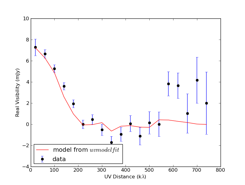
This CASA guide illustrates how to run UVMODELFIT to fit a single Gaussian component to UV data (i.e. the raw visibilities); and subsequently how to make a plot of the binned, "azimuthally" averaged (in UV space) UV data together with the fitted model. In broad outlines, the steps required are:
  1 Estimate the peak location of emission. shift the phase center here if desired.
  2 Estimate starting values for the gaussian component fit
  3 do the fit.
  4 run ft() to put the results of the fit in the MS explicitly (as a MODEL column).
  5 Extract MODEL and DATA, make the plot
The optional first step is to shift the phase center of the visibility data to the peak of emission in the map. This will maximize the amplitude of the azimuthally averaged profile in UV space, but is not strictly necessary for the results to be correct. This can be done using FIXVIS() --
fixvis(vis="J04292165_cont.ms",outputvis="J04292165_cont_recenter.ms",field="",refcode="",reuse=True,phasecenter="J2000 4h29m21.66s +27d01m25.72s",datacolumn="all")
(note: we have not actually done this stip in this example)
Next we fit a Gaussian component to the visibilities using UVMODELFIT(). Note that UVMODELFIT is currently restricted to fitting a single component. Since in general this is a nonlinear fit-- with no unique best-fit guarantee-- it is important that the initial values (SOURCEPAR) be set based on an initial inspection of the data.
default uvmodelfit
vis=myvis
field='0'
comptype='G'
sourcepar=[0.006,0.1,-0.05,0.4,0.3,0.0]
varypar=[]
outfile='J04292165_cont_allspw.uv.cl'
inp
go
again, in this example we had not phase shifted to the peak; otherwise we would have put "0,0" for the initial component center given by the "0.1,-0.05" [arcsec] entries of the SOURCEPAR parameters. The result of the UVMODELFIT is stored in a "component list", which can be used for various subsequent operations in CASA such as self-calibration.
In our case we simply wish to plot the visibilites that correspond to the best-fit (image domain) Gaussian model. This can be done by running the task FT to fourier transform the component list into the visibility domain. We will store the results in the MODEL column of the MS.
default ft
vis=myvis
complist='J04292165_cont_allspw.uv.cl'
usescratch=True
inp
go

# did that work?
plotms(vis=myvis,xaxis='uvwave',yaxis='real',ydatacolumn='model')
# yes it did.
By setting "usescratch=True" we ensured that the model visibilities are explicitly stored in the MS rather than using a a more compact implicit (reconstructed on-the-fly) representation -- the implicit representation does not work for the low level operations we wish to do.
Finally, use VISSTAT() to extract model and data values in bins of uv-radius:
# plotting script
#  KWD & JP Jul 2015

import numpy as np
import matplotlib.pyplot as plt
import glob

testms = 'J04292165_cont.ms'

# set the uvrange in kilo lambda
#  NB: take care that the bin width and uvmin/max ranges ensure
#   you get no bins without data! the appropriate values may change
#   if you, e.g., change the SPW you are looking at
uvmin = 0
#uvmax = 1200
uvmax = 800
 # define steps in klambda
duv=40

uvsteps = np.arange(uvmin, uvmax, duv)

avg_amps = [] # define an empty list in which to put the averaged amplitudes

stddev_amps = [] # define an empty list in which to put the amp stddev

numpoints = []

uvpoints = uvsteps[:-1] + np.diff(uvsteps)/2 # get array of uvmidpoints over which avg taken

model_amps = [] # define list to get model amplitudes after fourier transforming into the model data column

# iterate over the uvrange & build up
#  the binned data values (looking only at the Real part -- a pretty
#  good approach if the signal is approximately symmetric and you have
#  recentered the phase center on the peak of emission):
for ii in range(len(uvsteps[:-1])):
        tmp = visstat(vis = testms,axis = 'real',
                      uvrange = str(uvsteps[ii]) + '~' + str(uvsteps[ii+1]) + 'klambda',
                      datacolumn = 'data')
        print str(uvsteps[ii]) + '~' + str(uvsteps[ii+1]) + 'klambda'
        avg_amps.append(tmp['DATA']['mean'])
        stddev_amps.append(tmp['DATA']['stddev'])
        numpoints.append(tmp['DATA']['npts'])

# now build up the model values
for ii in range(len(uvsteps[:-1])):
        tmp = visstat(vis = testms,
                        axis = 'real', # you may want to change this to real...?
                        uvrange = str(uvsteps[ii]) + '~' + str(uvsteps[ii+1]) + 'klambda',
                        datacolumn = 'model')
        print str(uvsteps[ii]) + '~' + str(uvsteps[ii+1]) + 'klambda, from the model column'
        model_amps.append(tmp['MODEL']['mean'])

error_amps = stddev_amps/(np.sqrt(numpoints) - 1)

plt.clf()
plt.cla()

avg_amps_mjy = [x * 1000 for x in avg_amps]
model_amps_mjy = [x * 1000 for x in model_amps]
error_amps_mjy = [x * 1000 for x in error_amps]

plt.errorbar(uvpoints, avg_amps_mjy, yerr = error_amps_mjy, mfc='k', fmt='o', label='data')
plt.plot(uvpoints, model_amps_mjy, 'r-', label=r'model from $uvmodelfit$')

plt.legend(loc = 3, numpoints = 1)

plt.xlabel(r'UV Distance (k$\lambda$)')
plt.ylabel('Real Visibility (mJy)')

plt.show()
The resulting plot --
