Einstein-Face (CASA 3.4)
↵ Simulating Observations in CASA
This guide is applicable to CASA version 3.4. For simulation instructions for older versions of CASA see: Einstein-Face (CASA 3.3).
Simulations using non-science images: the face of Einstein
simobserve can be used to simulate any digitized image, while simanalyze can be used to image and analyze simulated data. These toy models can be particularly useful for examining the effects of varying uv-coverage on image fidelity if the "truth" model is a familiar object or image. In this example we use the face of Albert Einstein.
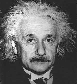
In this example, we grabbed a JPG image of Einstein's face from the internet. simobserve likes input images in fits format, so we used Gimp to convert the file. (Instructions to Convert jpg to fits.) The original image is shown below. You can grab the converted fits file here from the Simulation Inputs CASA Guide page.
Prepare inputs for simobserve and simanalyze
Start with the 10min full science observation. Inputs to simobserve and simanalyze are given below. The integration time is set much longer than realistic (300s, compared to 1-10s in practice) to speed the computation. The map spacing is set to ensure that only one pointing is observed. The image scale is chosen to ensure good sampling of the beam, and the observation is pointed near the Chandra Deep Field South:
# simobserve is used to simulate the observation
default 'simobserve'
# Full science, configuration 08, 10 minutes
project = 'fs_cfg8_10m'
skymodel = 'Einstein.fits'
indirection = 'J2000 03h30m00 -28d00m00'
incell = '0.043arcsec'
incenter = '245GHz'
inwidth = '2GHz'
setpointings = T
integration = '300s'
mapsize = ['1arcmin','1arcmin']
maptype = 'hexagonal'
pointingspacing = '1arcmin'
graphics = 'both'
Antenna configuration: ALMA antenna configuration files are stored in a directory found in the CASA installation. Details on configuration choices are given in the M51 simulation guide [1].
obsmode = 'int'
antennalist =  "alma.out08.cfg"
totaltime = '600s'
thermalnoise = ""
simobserve()
# simanalyze is used to take the simulation output, and provide helpful plots
default 'simanalyze'
project = 'fs_cfg8_10m'
image = T
vis = project+'.alma.out08.ms'
imsize = [300,300]
cell = '0.043arcsec'
niter = 2000
weighting = 'natural'
analyze = F
overwrite = T
simanalyze()
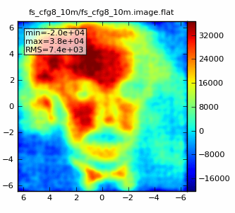
The output image should have a clean beam of 0.62"x0.56" and look something like:
Now we repeat for an 1hr observation:
tget simobserve
# Full science, configuration 08, 1 hour
project = 'fs_cfg8_1hr'
totaltime = '3600s'
simobserve()
tget simanalyze
project = 'fs_cfg8_1hr'
vis = project+'.alma.out08.ms'
simanalyze()
Which should look something like: 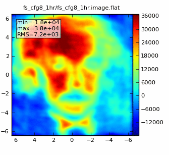
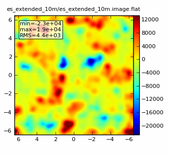
Finally, two Early Science simulations, using the extended configuration. One 10min simulation:
tget simobserve
project = 'es_extended_10m'
antennalist = "alma.cycle0.extended.cfg"
totaltime = '600s'
simobserve()
tget simanalyze
project = 'es_extended_10m'
vis = project+'.alma.cycle0.extended.ms'
simanalyze()
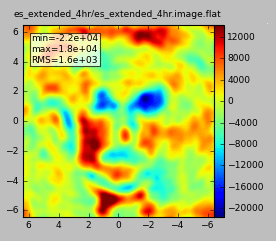
and a 4hr simulation:
tget simobserve
project = 'es_extended_4hr'
totaltime = '14400s'
simobserve()
tget simanalyze
project = 'es_extended_4hr'
vis = project+'.alma.cycle0.extended.ms'
simanalyze()
Further experiments:
Some more things to try:
An 8hr observation shows the improvement obtained by obtaining fuller uv-coverage in the full science array:
tget simobserve
antennalist = "alma.out08.cfg"
project = 'fs_cfg8_8hr'
totaltime = '28800s'
simobserve()
tget simanalyze
project = 'fs_cfg8_8hr'
vis = project+'.alma.out08.ms'
simanalyze()
Which should look something like: 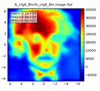
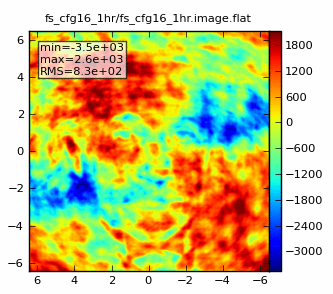
An attempt to make a higher resolution image shows what happens when short spacings are missing in the configuration. Configuration 16 has a 0.17x0.15 beam, still better than Nyquist sampling of the model image (which has 0.043" pixels). However, the lack of short spacings in the configuration leads to poorly sampled structure on large spatial scales. In practice, one would need to combine these observations with a set in a more compact configuration (such as 8) to sample both the large and small spatial structures.
tget simobserve
antennalist = "alma.out16.cfg"
project = 'fs_cfg16_1hr'
totaltime = '3600s'
simobserve()
tget simanalyze
project = 'fs_cfg16_1hr'
vis = project+'.alma.out16.ms'
simanalyze()
↵ Simulating Observations in CASA
Last checked on CASA Version 3.4.0.
