VLBA Basic Phase-referencing Calibration and Imaging: Difference between revisions
| (17 intermediate revisions by the same user not shown) | |||
| Line 12: | Line 12: | ||
* Astrometric — Earth orientation parameter (EOP) and pulse-cal tone corrections are not yet available in CASA. | * Astrometric — Earth orientation parameter (EOP) and pulse-cal tone corrections are not yet available in CASA. | ||
* Spectral line projects requiring fringe-rate mapping — Fringe-rate mapping is not yet available in CASA. | * Spectral line projects requiring fringe-rate mapping — Fringe-rate mapping is not yet available in CASA. | ||
* Low Frequency (<4 GHz) — Total electron content (TEC) corrections have not yet been verified to work correctly for VLBI observations in CASA. | * Low Frequency (<4 GHz) — Total electron content (TEC) corrections have not yet been verified to work correctly for VLBI observations in CASA. Also, note that many C-band (4 to 8 GHz) VLBA observations will benefit from TEC corrections. | ||
* VLBA+Y27 or other VLBA+ arrays that require the use of antab files — CASA does not currently support the use of antab files for ingesting calibration data (system temperatures, gain curves, etc.) | |||
* VLBA data correlated prior to December 2009 — CASA cannot load data correlated with the old VLBA hardware correlator. Your data must have been correlated with the [https://go.nrao.edu/difx DiFX correlator]. | |||
If your observation involves any of the above, you should use [http://www.aips.nrao.edu/index.shtml AIPS] to calibrate your data. | If your observation involves any of the above, you should use [http://www.aips.nrao.edu/index.shtml AIPS] to calibrate your data. | ||
<b>A note on VLBA+Y1 observations:</b> It is currently possible to calibrate VLBA+Y1 (VLBA and single VLA antenna) in CASA. Any data taken after 2022 July 06 should work with minimal extra steps (namely, checking that the Y1 antenna diameter is correct). VLBA+Y1 data observed prior to 2022 July 06 may not include the system temperature and/or gain | <b>A note on VLBA+Y1 observations:</b> It is currently possible to calibrate VLBA+Y1 (VLBA and single VLA antenna) in CASA. Any data taken after 2022 July 06 should work with minimal extra steps (namely, checking that the Y1 antenna diameter is correct). VLBA+Y1 data observed prior to 2022 July 06 may not include the system temperature and/or gain curve values need for calibration. For these data sets, refer to [https://library.nrao.edu/public/memos/vlba/sci/VLBAS_39.pdf VLBA Scientific Memo 39] for details on how to prepare the data for calibration in either CASA or AIPS. | ||
== How to Use This CASA Guide == | == How to Use This CASA Guide == | ||
| Line 40: | Line 40: | ||
Alternatively, you may download the data from the [https://data.nrao.edu NRAO Archive]. In the archive search inputs, enter "TL016" in the Project Code field. Expand the results for TL016B and look for the file VLBA_TL016B_tl016b_BIN0_SRC0_1_220307T210851.idifits. Select the file, click "Download", and follow the instructions. Once you have downloaded the FITS-IDI file from the archive, it will be helpful to change the filename to "TL016B.idifits". | Alternatively, you may download the data from the [https://data.nrao.edu NRAO Archive]. In the archive search inputs, enter "TL016" in the Project Code field. Expand the results for TL016B and look for the file VLBA_TL016B_tl016b_BIN0_SRC0_1_220307T210851.idifits. Select the file, click "Download", and follow the instructions. Once you have downloaded the FITS-IDI file from the archive, it will be helpful to change the filename to "TL016B.idifits". | ||
== The | == The Observing Log == | ||
Before diving into the calibration, it is always a good idea to look over the observing log to | Before diving into the calibration, it is always a good idea to look over the observing log to check for notes from the operators that can inform us about potential issues with the data (missing stations, bad weather, etc.). These logs are always emailed to the PI's of an observation, but you can also access them later from the NRAO's [http://www.vlba.nrao.edu/astro/VOBS/astronomy/ vlbiobs fileserver]. To locate an observing log, first find the directory for observing month and the last two digits of the year (for the observation used in this Guide, that directory is [http://www.vlba.nrao.edu/astro/VOBS/astronomy/feb22/ feb22] for February 2022). Once inside the proper month+year directory, look for the project code (in this case, [http://www.vlba.nrao.edu/astro/VOBS/astronomy/feb22/tl016b/ tl016b]). Look for a file named <project code>log.vbla ([http://www.vlba.nrao.edu/astro/VOBS/astronomy/feb22/tl016b/tl016blog.vlba tl016blog.vlba]). | ||
The observing log for this particular observation looked like this: | The observing log for this particular observation looked like this: | ||
| Line 103: | Line 103: | ||
</source> | </source> | ||
The ''scanreindexgap_s'' parameter is used to reconstruct scan boundaries in those cases where sources do not change between scans. In general, it is good to set ''scanreindexgap_s'' to some non-zero number to help CASA properly organize the scan list. The recommended value is 15, but shorter values may work as well (although you probably don't want to go much shorter than about 5 seconds). If you find that the resulting MS contains too few scans, run [https://casadocs.readthedocs.io/en/v6.4.0/api/tt/casatasks.data.importfitsidi.html importfitsidi] again with ''scanreindexgap_s'' set to a smaller number. If your MS has too many scans, especially multiple scans on the same source when you think it should just be one scan, run [https://casadocs.readthedocs.io/en/v6.4.0/api/tt/casatasks.data.importfitsidi.html importfitsidi] again with ''scanreindexgap_s'' set to a larger number. | The ''scanreindexgap_s'' parameter is used to reconstruct scan boundaries in those cases where sources do not change between scans. In general, it is good to set ''scanreindexgap_s'' to some non-zero number to help CASA properly organize the scan list. The recommended value is 15 seconds, but shorter values may work as well (although you probably don't want to go much shorter than about 5 seconds). If you find that the resulting MS contains too few scans, run [https://casadocs.readthedocs.io/en/v6.4.0/api/tt/casatasks.data.importfitsidi.html importfitsidi] again with ''scanreindexgap_s'' set to a smaller number. If your MS has too many scans, especially multiple scans on the same source when you think it should just be one scan, run [https://casadocs.readthedocs.io/en/v6.4.0/api/tt/casatasks.data.importfitsidi.html importfitsidi] again with ''scanreindexgap_s'' set to a larger number. | ||
<b> NOTE: </b>You may see warnings in the CASA window like "Table not yet implemented" and "Keyword has wrong data type". This is normal behavior for VLBA data and due to the fact that CASA does not yet handle the pulse-cal tone data in the FTIS-IDI file. Just ignore them. | <b> NOTE: </b>You may see warnings in the CASA window like "Table not yet implemented" and "Keyword has wrong data type". This is normal behavior for VLBA data and due to the fact that CASA does not yet handle the pulse-cal tone data in the FTIS-IDI file. Just ignore them. However, do not ignore any SEVERE warnings, as these can indicate there are serious problems with the data. | ||
== Inspecting the Data == | == Inspecting the Data == | ||
| Line 406: | Line 406: | ||
VLBA calibration makes use of a reference antenna: one antenna that all other antennas can be referenced to when generating solutions. Usually, you will want to use one of the more central stations: FD, KP, LA, or PT. | VLBA calibration makes use of a reference antenna: one antenna that all other antennas can be referenced to when generating solutions. Usually, you will want to use one of the more central stations: FD, KP, LA, or PT. | ||
To determine which is the best to use as the reference antenna, use [https://casadocs.readthedocs.io/en/v6.4.0/api/tt/casaplotms.plotms.html plotms] to plot phase vs frequency for a single scan on a bright source (usually the fringe finder or bandpass calibrator). For this observation, use the third scan on 4C39.25, which is scan 91 from the | To determine which is the best to use as the reference antenna, use [https://casadocs.readthedocs.io/en/v6.4.0/api/tt/casaplotms.plotms.html plotms] to plot phase vs frequency for a single scan on a bright source (usually the fringe finder or bandpass calibrator). For this observation, use the third scan on 4C39.25, which is scan 91 from the [https://casadocs.readthedocs.io/en/v6.4.0/api/tt/casatasks.information.listobs.html listobs] output. Inspect each of the 4 central antennas and use the one which has the most well-behaved phases. We start with scan 91 because it is near the middle of our observation, so 4C39.25 should be at relatively high elevations at all stations during that scan. | ||
<b> NOTE: </b> For our observation, we know that it was windy at KP so we probably do not want to use that one as the reference antenna. | <b> NOTE: </b> For our observation, we know that it was windy at KP so we probably do not want to use that one as the reference antenna. | ||
| Line 417: | Line 417: | ||
Use the GUI to step though the baselines. Look at each antenna and look at both right- and left-hand polarization (''correlation='rr' '' and ''correlation='ll' ''). Our observation does not include the cross-hand polarizations (lr and rl), and you usually won't worry about inspecting them anyway since they will usually be too low to see anything useful. | Use the GUI to step though the baselines. Look at each antenna and look at both right- and left-hand polarization (''correlation='rr' '' and ''correlation='ll' ''). Our observation does not include the cross-hand polarizations (lr and rl), and you usually won't worry about inspecting them anyway since they will usually be too low to see anything useful. | ||
In the GUI, go to the "Axes" tab and change the "Data" axis to "Amp" (this is equivalent to settining ''yaxis='amplitude''') to inspect the shapes of the bandpasses and look for RFI. If antenna has strong RFI, you should not use it as the reference antenna. | In the GUI, go to the "Axes" tab and change the "Data" axis to "Amp" (this is equivalent to settining ''yaxis='amplitude''') to inspect the shapes of the bandpasses and look for RFI. If an antenna has strong RFI, you should not use it as the reference antenna. | ||
For this observation, we will use Fort Davis (FD) as the reference antenna. Its phases are fairly smooth, it is free of RFI, and the bandpasses look pretty clean (especially compared to PT in spw 2 and 3). | For this observation, we will use Fort Davis (FD) as the reference antenna. Its phases are fairly smooth, it is free of RFI, and the bandpasses look pretty clean (especially compared to PT in spw 2 and 3). | ||
| Line 523: | Line 523: | ||
|} | |} | ||
Flag all | Flag all baselines to HN on the final scan of 4C39.25 using [https://casadocs.readthedocs.io/en/v6.4.0/api/tt/casatasks.flagging.flagdata.html flagdata]. | ||
<source lang="python"> | <source lang="python"> | ||
#In CASA | #In CASA | ||
| Line 718: | Line 718: | ||
Spw 3: 1/1/1 | Spw 3: 1/1/1 | ||
</pre> | </pre> | ||
This is exactly what we expect to see. We are | This is exactly what we expect to see. We are only attempting to get one solution per spw because we are only solving over a single solution interval (one minute of data from a single scan). | ||
Apply the instrumental delay corrections using [https://casadocs.readthedocs.io/en/v6.4.0/api/tt/casatasks.calibration.applycal.html applycal]. | Apply the instrumental delay corrections using [https://casadocs.readthedocs.io/en/v6.4.0/api/tt/casatasks.calibration.applycal.html applycal]. | ||
| Line 838: | Line 838: | ||
It will probably take a while for [https://casadocs.readthedocs.io/en/v6.4.0/api/tt/casatasks.calibration.applycal.html applycal] to run again, since you are also applying the solutions from the global fringe fitting. | It will probably take a while for [https://casadocs.readthedocs.io/en/v6.4.0/api/tt/casatasks.calibration.applycal.html applycal] to run again, since you are also applying the solutions from the global fringe fitting. | ||
After | After applying the bandpass solutions, take a look at the calibrated data with [https://casadocs.readthedocs.io/en/v6.4.0/api/tt/casaplotms.plotms.html plotms]. | ||
<source lang="python"> | <source lang="python"> | ||
#In CASA | #In CASA | ||
| Line 846: | Line 846: | ||
The bands look pretty good, but there is some offset between the bands and between polarizations ("correlations") inside each band. This is usually not a big deal and can be corrected with self-calibration. | The bands look pretty good, but there is some offset between the bands and between polarizations ("correlations") inside each band. This is usually not a big deal and can be corrected with self-calibration. | ||
The bandpass calibration often does not perfectly calibrate the channels at the beginning and end of each spectral window. We can see such problems in | The bandpass calibration often does not perfectly calibrate the channels at the beginning and end of each spectral window. We can see such problems in our data where there are often outliers (both high and low) at the edges of each band. It is often a good idea to get rid of the edge channels that are not well-calibrated. We will use [https://casadocs.readthedocs.io/en/v6.4.0/api/tt/casatasks.flagging.flagdata.html flagdata] to get rid of some of the edge channels. | ||
For our data, we will flag the first and last 3 channels of each spw. | For our data, we will flag the first and last 3 channels of each spw. | ||
| Line 912: | Line 912: | ||
Despite our best efforts with the initial calibration, VLBA observations will almost always require additional steps to improve the calibration. Because the VLBA antennas are separated by such large distances, the phases may not be perfectly calibrated by fringe fitting alone. This is partly because each antenna may be looking through vastly different troposphere/ionosphere, and partly because the phase reference calibrators are rarely point sources on long baselines (and fringe-fitting usually assumes the calibrators are point sources on all baselines). | Despite our best efforts with the initial calibration, VLBA observations will almost always require additional steps to improve the calibration. Because the VLBA antennas are separated by such large distances, the phases may not be perfectly calibrated by fringe fitting alone. This is partly because each antenna may be looking through vastly different troposphere/ionosphere, and partly because the phase reference calibrators are rarely point sources on long baselines (and fringe-fitting usually assumes the calibrators are point sources on all baselines). | ||
We will improve the calibration using "self-calibration". The process of self-calibration involves building models of the sources, refining the calibration based on those models, and then repeating until you converge to a good solution. The models are created during the imaging process. Each iteration self-calibration should produce images with lower noise. | We will improve the calibration using "self-calibration". The process of self-calibration involves building models of the sources, refining the calibration based on those models, and then repeating until you converge to a good solution. The models are created during the imaging process. Each iteration of self-calibration should produce images with lower noise. | ||
Each time the noise is reduced, you may notice dimmer structures appear. This is where you need to be careful. Including an apparent structure in a model for self-calibration can "build in" features that are not real. A good rule of thumb is "if you can't self-calibrate a structure away, it is probably real". So, if you are uncertain whether a newly apparent component is real or not, first try to self-calibrate without including that component in the model. If it sticks around, it is probably a real structure and including it in the next model should further improve the calibration and lower the noise in the next image. | Each time the noise is reduced, you may notice dimmer structures appear. This is where you need to be careful. Including an apparent structure in a model for self-calibration can "build in" features that are not real. A good rule of thumb is "if you can't self-calibrate a structure away, it is probably real". So, if you are uncertain whether a newly apparent component is real or not, first try to self-calibrate without including that component in the model. If it sticks around, it is probably a real structure and including it in the next model should further improve the calibration and lower the noise in the next image. | ||
| Line 959: | Line 959: | ||
Setting ''interactive=True'' will allow us to define the areas where there is real flux from the source ("clean windows"). The value for ''niter'' needs to be large enough that we can go through enough clean iterations to recover most of the source flux. You can set ''niter'' to any arbitrarily large number (a few hundred should be plenty), but 1000 is an easy value to remember. Setting ''savemodel='modelcolumn' '' will save the model we create for the image to the model column of the measurement set so we can use it for self-calibration. | Setting ''interactive=True'' will allow us to define the areas where there is real flux from the source ("clean windows"). The value for ''niter'' needs to be large enough that we can go through enough clean iterations to recover most of the source flux. You can set ''niter'' to any arbitrarily large number (a few hundred should be plenty), but 1000 is an easy value to remember. Setting ''savemodel='modelcolumn' '' will save the model we create for the image to the model column of the measurement set so we can use it for self-calibration. | ||
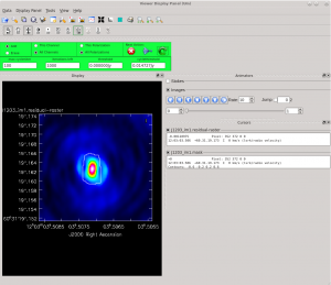
Running [https://casadocs.readthedocs.io/en/v6.4.0/api/tt/casatasks.imaging.tclean.html tclean] with ''interactive=True'' will open a new Viewer Display Panel where you can control the cleaning of the image. You should see that J1154+6022 is fairly point-like. Use the zoom tool to select the region | Running [https://casadocs.readthedocs.io/en/v6.4.0/api/tt/casatasks.imaging.tclean.html tclean] with ''interactive=True'' will open a new Viewer Display Panel where you can control the cleaning of the image. You should see that J1154+6022 is fairly point-like. Use the zoom tool to select the region around the source. Use the "polygon drawing" tool to draw a clean window around the source, excluding the stuff to the left and right of the bright source. Click on the "Continue deconvolution" button (the green circular arrow on the right). Check the residuals when the display updates. Stop cleaning when the area around the source looks noise-like. For example, if you notice positive and negative regions with similar magnitudes (e.g., +0.003 and -0.003) inside your clean window, that is probably a good time to stop cleaning. To stop the cleaning process, click the "stop deconvolving now" button (the red circle with the white "X"). It may take [https://casadocs.readthedocs.io/en/v6.4.0/api/tt/casatasks.imaging.tclean.html tclean] a while to finish and close. | ||
<b>NOTE: </b>If you need to delete a clean window, select "Erase" at the far left of the green region in the GUI and draw a box around the clean window(s) you want to delete, then double click. Remember to select "Add" again to define new clean windows. | <b>NOTE: </b>If you need to delete a clean window, select "Erase" at the far left of the green region in the GUI and draw a box around the clean window(s) you want to delete, then double click. Remember to select "Add" again to define new clean windows. | ||
| Line 1,073: | Line 1,073: | ||
Notice that when refining both the delays and the phases we set ''minblperant=3'' because closure phases require at least 3 baselines. | Notice that when refining both the delays and the phases we set ''minblperant=3'' because closure phases require at least 3 baselines. | ||
Apply the phase self-calibration | Apply the phase self-calibration solutions to the phase reference calibrator. | ||
<source lang="python"> | <source lang="python"> | ||
#In CASA | #In CASA | ||
| Line 1,133: | Line 1,133: | ||
Writing solutions to table: tl016b_cal1.apcal | Writing solutions to table: tl016b_cal1.apcal | ||
</pre> | </pre> | ||
The mean normalization factors are all close to 1.0, which is what we expect since we set ''solnorm=True''. If the mean values were far from 1.0, we would be worried that the amplitude self-calibration was not working properly (perhaps one or | The mean normalization factors are all close to 1.0, which is what we expect since we set ''solnorm=True''. If the mean values were far from 1.0, we would be worried that the amplitude self-calibration was not working properly (perhaps one or two of the antennas were drastically low or high). | ||
We should also take a look at the solutions on each telescope using [https://casadocs.readthedocs.io/en/v6.4.0/api/tt/casaplotms.plotms.html plotms]. | We should also take a look at the solutions on each telescope using [https://casadocs.readthedocs.io/en/v6.4.0/api/tt/casaplotms.plotms.html plotms]. | ||
Latest revision as of 12:26, 26 September 2023
This CASA Guide is for Version 6.4.0 of CASA. If you are using a later version of CASA and this is the most recent available guide, then you should be able to use most, if not all, of this tutorial.
Overview
This CASA Guide describes the procedure for calibrating a phase-referenced VLBA observation of the radio galaxy J1203+6031 (IVS 1200+608, ICRF3 J120303.5+603119). The data were taken specifically for this tutorial. The observation made use of the DDC observing personality, using dual polarization with 4 spectral windows per polarization. Each spectral window is has a bandwidth of 64 MHz, and is divided into 128 spectral channels.
This tutorial will focus on calibrating the data and creating continuum (Stokes I) images.
Please note that CASA should be used with caution when calibrating VLBA data. At the current time, CASA should only be used to calibrate relatively simple VLBA observations (basic continuum, simple phase-referenced, etc.). In particular, CASA is currently not recommended for calibrating the following types of VLBA observations:
- Polarimetric — Calibration of resolved polarized sources is not yet available in CASA.
- Astrometric — Earth orientation parameter (EOP) and pulse-cal tone corrections are not yet available in CASA.
- Spectral line projects requiring fringe-rate mapping — Fringe-rate mapping is not yet available in CASA.
- Low Frequency (<4 GHz) — Total electron content (TEC) corrections have not yet been verified to work correctly for VLBI observations in CASA. Also, note that many C-band (4 to 8 GHz) VLBA observations will benefit from TEC corrections.
- VLBA+Y27 or other VLBA+ arrays that require the use of antab files — CASA does not currently support the use of antab files for ingesting calibration data (system temperatures, gain curves, etc.)
- VLBA data correlated prior to December 2009 — CASA cannot load data correlated with the old VLBA hardware correlator. Your data must have been correlated with the DiFX correlator.
If your observation involves any of the above, you should use AIPS to calibrate your data.
A note on VLBA+Y1 observations: It is currently possible to calibrate VLBA+Y1 (VLBA and single VLA antenna) in CASA. Any data taken after 2022 July 06 should work with minimal extra steps (namely, checking that the Y1 antenna diameter is correct). VLBA+Y1 data observed prior to 2022 July 06 may not include the system temperature and/or gain curve values need for calibration. For these data sets, refer to VLBA Scientific Memo 39 for details on how to prepare the data for calibration in either CASA or AIPS.
How to Use This CASA Guide
There are a number of possible ways to run CASA, described in more detail in Getting Started in CASA. In brief, there are at least three different ways to use CASA:
- Interactively examining task inputs. In this mode, one types taskname to load the task, inp to examine the inputs, and go once those inputs have been set to your satisfaction. Allowed inputs are shown in blue and bad inputs are colored red. The input parameters themselves are changed one by one, e.g., selectdata=True. Screenshots of the inputs to various tasks used in the data reduction below are provided, to illustrate which parameters need to be set. More detailed help can be obtained on any task by typing help taskname. Once a task is run, the set of inputs are stored and can be retrieved via tget taskname; subsequent runs will overwrite the previous tget file.
- Pseudo-interactively via task function calls. In this case, all of the desired inputs to a task are provided at once on the CASA command line. This tutorial is made up of such calls, which were developed by looking at the inputs for each task and deciding what needed to be changed from default values. For task function calls, only parameters that you want to be different from their defaults need to be set.
- Non-interactively via a script. A series of task function calls can be combined together into a script, and run from within CASA via execfile('scriptname.py'). This and other CASA Tutorial Guides have been designed to be extracted into a script via the script extractor by using the method described at the Extracting_scripts_from_these_tutorials page. Should you use the script generated by the script extractor for this CASA Guide, be aware that it will require some small amount of interaction related to the plotting, occasionally suggesting that you close the graphics window and hitting return in the terminal to proceed. It is in fact unnecessary to close the graphics windows (it is suggested that you do so purely to keep your desktop uncluttered).
If you are a relative novice or just new to CASA, it is strongly recommended to work through this tutorial by cutting and pasting the task function calls provided below after you have read all the associated explanations. Work at your own pace, look at the inputs to the tasks to see what other options exist, and read the help files. Later, when you are more comfortable, you might try to extract the script, modify it for your purposes, and begin to reduce other data.
NOTE: It is not recommended to use scripts to generate "science-ready" VLBA data products. Nearly all VLBA observations will require some amount of hands-on calibration. Calibration and imaging scripts should only be used as "first pass" attempts at calibration, which can be useful to determine if the observation resulted in a detection and to identify problems in the data.
Obtaining the Data
This Guide is intended to cover the entire process one would follow for calibrating their own VLBA observation. Therefore, we will start with a FITS-IDI file rather than a Measurement Set. The FITS-IDI file for this Guide is: TL016B.idifits (right-click and select "Save Link As..."; file size: 3.8 GB).
Alternatively, you may download the data from the NRAO Archive. In the archive search inputs, enter "TL016" in the Project Code field. Expand the results for TL016B and look for the file VLBA_TL016B_tl016b_BIN0_SRC0_1_220307T210851.idifits. Select the file, click "Download", and follow the instructions. Once you have downloaded the FITS-IDI file from the archive, it will be helpful to change the filename to "TL016B.idifits".
The Observing Log
Before diving into the calibration, it is always a good idea to look over the observing log to check for notes from the operators that can inform us about potential issues with the data (missing stations, bad weather, etc.). These logs are always emailed to the PI's of an observation, but you can also access them later from the NRAO's vlbiobs fileserver. To locate an observing log, first find the directory for observing month and the last two digits of the year (for the observation used in this Guide, that directory is feb22 for February 2022). Once inside the proper month+year directory, look for the project code (in this case, tl016b). Look for a file named <project code>log.vbla (tl016blog.vlba).
The observing log for this particular observation looked like this:
VERY LONG BASELINE ARRAY OBSERVING LOG
--------------------------------------
Project:        TL016B
Observer:       Linford, J.
Project type:   VLBA
Obs filename:   t;016b.vex
Date/Day:       2022FEB21/052
Ants Scheduled: SC HN NL FD LA PT KP OV BR MK

=UT-Time===Comment===============================================MF#===%AD==AMD=
           Operator is Betty Ragan
     0559  Begin
     0559 %SC raining
     0559 %KP windy
     1327  End.


Downtime Summary:
	Total downtime : 0 min
	Percentage downtime of observing: 0.0%
	Average downtime per hour : 0.0 min

    Total scheduled observing time (# Antennas): 4480 min (10)

Notes:
    * = Entries where data was affected.
    % = Entries where data may have been affected.
    & = Entries where the site tech was called out.
  WEA = Weather entries.
  MF# = Maintenance form or major downtime category associated with a problem.
  %AD = The percentage of an antenna affected by a problem.
  AMD = Total antenna-minutes downtime for a problem.
 Tsys = System Temperature (TP/SP x Tcal/2)
  ACU = Antenna Control Unit
  FRM = Focus/Rotation Mount
  RFI = Radio Frequency Interference
  VME = Site control computer
   CB = Circuit Breaker
 vclock = Program that compares site clock time to a standard.
There are no major issues reported by the operators for this observation and all ten antennas participated for the entire time (no downtime). However, there was rain at Saint Croix (SC) and it was windy at Kitt Peak (KP). We'll need to keep that in mind as we proceed with the calibration. We should pay special attention to SC and KP as we inspect the data and the calibration solutions we generate.
NOTE: This is an exceptionally good observing log! Most observations will have at least a small amount of downtime for various reasons.
Creating the Measurement Set
Before beginning our data reduction, we must start CASA. If you have not used CASA before, some helpful tips are available on the Getting Started in CASA page. Remember to start CASA in the directory containing the observation data.
Once you have CASA up and running, it is time to get the data into a format that CASA can use. Unlike VLA data, a VLBA observation is only available as a FITS-IDI file and cannot be downloaded as a CASA Measurement Set. So, the first step in calibrating a VLBA observation with CASA is to create a Measurement Set from the FITS-IDI file. To do this, we will use the task importfitsidi:
# In CASA
importfitsidi(fitsidifile='TL016B.idifits', vis='tl016b.ms', constobsid=True, scanreindexgap_s=15)
The scanreindexgap_s parameter is used to reconstruct scan boundaries in those cases where sources do not change between scans. In general, it is good to set scanreindexgap_s to some non-zero number to help CASA properly organize the scan list. The recommended value is 15 seconds, but shorter values may work as well (although you probably don't want to go much shorter than about 5 seconds). If you find that the resulting MS contains too few scans, run importfitsidi again with scanreindexgap_s set to a smaller number. If your MS has too many scans, especially multiple scans on the same source when you think it should just be one scan, run importfitsidi again with scanreindexgap_s set to a larger number.
NOTE: You may see warnings in the CASA window like "Table not yet implemented" and "Keyword has wrong data type". This is normal behavior for VLBA data and due to the fact that CASA does not yet handle the pulse-cal tone data in the FTIS-IDI file. Just ignore them. However, do not ignore any SEVERE warnings, as these can indicate there are serious problems with the data.
Inspecting the Data
Now that we have a Measurement Set, it is time to look over the data, identify a good reference antenna, and find a good time range to use for calibrating the instrumental delay.
The Observation Summary
It will be useful later to have the basic information about the observation. The task listobs will return a list of all the scans, the sources observed, which stations were used, and the frequency setup. It is possible to run listobs in two ways: printing information in the CASA logger, or saving the information to a file.
To simply display the information in the CASA logger:
#In CASA
listobs(vis='tl016b.ms')
You should see the listobs output in the CASA logger window:
================================================================================
MeasurementSet Name: tl016b.ms MS Version 2
================================================================================
Observer: PLUTO Project: TL016B
Observation: VLBA
Data records: 1992052 Total elapsed time = 26010 seconds
Observed from 21-Feb-2022/06:13:39.0 to 21-Feb-2022/13:27:09.0 (UTC)
ObservationID = 0 ArrayID = 0
Date Timerange (UTC) Scan FldId FieldName nRows SpwIds Average Interval(s) ScanIntent
21-Feb-2022/06:13:39.0 - 06:17:09.0 1 0 4C39.25 23100 [0,1,2,3] [2, 2, 2, 2]
06:18:34.0 - 06:19:34.0 2 1 J1154+6022 6200 [0,1,2,3] [2, 2, 2, 2]
06:19:44.0 - 06:21:44.0 3 2 J1203+6031 13200 [0,1,2,3] [2, 2, 2, 2]
06:21:55.0 - 06:22:35.0 4 1 J1154+6022 4400 [0,1,2,3] [2, 2, 2, 2]
06:22:45.0 - 06:24:45.0 5 2 J1203+6031 13200 [0,1,2,3] [2, 2, 2, 2]
06:24:55.0 - 06:25:35.0 6 1 J1154+6022 4400 [0,1,2,3] [2, 2, 2, 2]
06:25:46.0 - 06:27:46.0 7 2 J1203+6031 13200 [0,1,2,3] [2, 2, 2, 2]
06:27:56.0 - 06:28:36.0 8 1 J1154+6022 4400 [0,1,2,3] [2, 2, 2, 2]
06:28:47.0 - 06:30:47.0 9 2 J1203+6031 13200 [0,1,2,3] [2, 2, 2, 2]
06:30:57.0 - 06:31:37.0 10 1 J1154+6022 4400 [0,1,2,3] [2, 2, 2, 2]
06:31:47.0 - 06:33:47.0 11 2 J1203+6031 13200 [0,1,2,3] [2, 2, 2, 2]
06:33:58.0 - 06:34:38.0 12 1 J1154+6022 4400 [0,1,2,3] [2, 2, 2, 2]
06:34:48.0 - 06:36:48.0 13 2 J1203+6031 13200 [0,1,2,3] [2, 2, 2, 2]
06:36:59.0 - 06:37:39.0 14 1 J1154+6022 4400 [0,1,2,3] [2, 2, 2, 2]
06:37:49.0 - 06:39:49.0 15 2 J1203+6031 13200 [0,1,2,3] [2, 2, 2, 2]
06:40:00.0 - 06:40:40.0 16 1 J1154+6022 4360 [0,1,2,3] [2, 2, 2, 2]
06:40:50.0 - 06:42:50.0 17 2 J1203+6031 13160 [0,1,2,3] [2, 2, 2, 2]
06:43:01.0 - 06:43:41.0 18 1 J1154+6022 4360 [0,1,2,3] [2, 2, 2, 2]
06:43:51.0 - 06:45:51.0 19 2 J1203+6031 13160 [0,1,2,3] [2, 2, 2, 2]
06:46:02.0 - 06:46:42.0 20 1 J1154+6022 4360 [0,1,2,3] [2, 2, 2, 2]
06:46:53.0 - 06:48:53.0 21 2 J1203+6031 13200 [0,1,2,3] [2, 2, 2, 2]
06:49:03.0 - 06:49:43.0 22 1 J1154+6022 4356 [0,1,2,3] [2, 2, 2, 2]
06:57:02.0 - 06:57:58.0 23 1 J1154+6022 5004 [0,1,2,3] [2, 2, 2, 2]
06:58:08.0 - 07:00:08.0 24 2 J1203+6031 13160 [0,1,2,3] [2, 2, 2, 2]
07:00:19.0 - 07:00:59.0 25 1 J1154+6022 4400 [0,1,2,3] [2, 2, 2, 2]
07:01:10.0 - 07:03:10.0 26 2 J1203+6031 13200 [0,1,2,3] [2, 2, 2, 2]
07:03:20.0 - 07:04:00.0 27 1 J1154+6022 4360 [0,1,2,3] [2, 2, 2, 2]
07:04:11.0 - 07:06:11.0 28 2 J1203+6031 13200 [0,1,2,3] [2, 2, 2, 2]
07:06:21.0 - 07:07:01.0 29 1 J1154+6022 4360 [0,1,2,3] [2, 2, 2, 2]
07:07:12.0 - 07:09:12.0 30 2 J1203+6031 13200 [0,1,2,3] [2, 2, 2, 2]
07:09:22.0 - 07:10:02.0 31 1 J1154+6022 4400 [0,1,2,3] [2, 2, 2, 2]
07:10:13.0 - 07:12:13.0 32 2 J1203+6031 13200 [0,1,2,3] [2, 2, 2, 2]
07:12:23.0 - 07:13:03.0 33 1 J1154+6022 4400 [0,1,2,3] [2, 2, 2, 2]
07:13:14.0 - 07:15:14.0 34 2 J1203+6031 13200 [0,1,2,3] [2, 2, 2, 2]
07:15:24.0 - 07:16:04.0 35 1 J1154+6022 4400 [0,1,2,3] [2, 2, 2, 2]
07:16:14.0 - 07:18:14.0 36 2 J1203+6031 13200 [0,1,2,3] [2, 2, 2, 2]
07:18:25.0 - 07:19:05.0 37 1 J1154+6022 4400 [0,1,2,3] [2, 2, 2, 2]
07:19:15.0 - 07:21:15.0 38 2 J1203+6031 13200 [0,1,2,3] [2, 2, 2, 2]
07:21:26.0 - 07:22:06.0 39 1 J1154+6022 4400 [0,1,2,3] [2, 2, 2, 2]
07:22:16.0 - 07:24:16.0 40 2 J1203+6031 13200 [0,1,2,3] [2, 2, 2, 2]
07:24:26.0 - 07:25:06.0 41 1 J1154+6022 4400 [0,1,2,3] [2, 2, 2, 2]
07:25:16.0 - 07:27:16.0 42 2 J1203+6031 13200 [0,1,2,3] [2, 2, 2, 2]
07:27:26.0 - 07:28:06.0 43 1 J1154+6022 4188 [0,1,2,3] [2, 2, 2, 2]
07:40:49.0 - 07:44:19.0 44 0 4C39.25 23100 [0,1,2,3] [2, 2, 2, 2]
07:46:03.0 - 07:47:03.0 45 1 J1154+6022 6200 [0,1,2,3] [2, 2, 2, 2]
07:47:12.0 - 07:49:12.0 46 2 J1203+6031 13200 [0,1,2,3] [2, 2, 2, 2]
07:49:22.0 - 07:50:02.0 47 1 J1154+6022 4400 [0,1,2,3] [2, 2, 2, 2]
07:50:12.0 - 07:52:12.0 48 2 J1203+6031 13020 [0,1,2,3] [2, 2, 2, 2]
07:52:22.0 - 07:53:04.0 49 1 J1154+6022 4440 [0,1,2,3] [2, 2, 2, 2]
07:53:13.0 - 07:55:13.0 50 2 J1203+6031 13020 [0,1,2,3] [2, 2, 2, 2]
07:55:23.0 - 07:56:03.0 51 1 J1154+6022 4220 [0,1,2,3] [2, 2, 2, 2]
07:56:13.0 - 07:58:15.0 52 2 J1203+6031 13240 [0,1,2,3] [2, 2, 2, 2]
07:58:24.0 - 07:59:04.0 53 1 J1154+6022 4240 [0,1,2,3] [2, 2, 2, 2]
07:59:14.0 - 08:01:14.0 54 2 J1203+6031 13040 [0,1,2,3] [2, 2, 2, 2]
08:01:24.0 - 08:02:06.0 55 1 J1154+6022 4620 [0,1,2,3] [2, 2, 2, 2]
08:02:15.0 - 08:04:15.0 56 2 J1203+6031 13200 [0,1,2,3] [2, 2, 2, 2]
08:04:25.0 - 08:05:07.0 57 1 J1154+6022 4620 [0,1,2,3] [2, 2, 2, 2]
08:05:16.0 - 08:07:16.0 58 2 J1203+6031 13200 [0,1,2,3] [2, 2, 2, 2]
08:07:26.0 - 08:08:06.0 59 1 J1154+6022 4400 [0,1,2,3] [2, 2, 2, 2]
08:08:16.0 - 08:10:18.0 60 2 J1203+6031 12060 [0,1,2,3] [2, 2, 2, 2]
08:10:27.0 - 08:11:07.0 61 1 J1154+6022 4240 [0,1,2,3] [2, 2, 2, 2]
08:11:17.0 - 08:13:17.0 62 2 J1203+6031 13064 [0,1,2,3] [2, 2, 2, 2]
08:13:27.0 - 08:14:09.0 63 1 J1154+6022 4484 [0,1,2,3] [2, 2, 2, 2]
08:14:18.0 - 08:16:18.0 64 2 J1203+6031 13064 [0,1,2,3] [2, 2, 2, 2]
08:16:28.0 - 08:17:10.0 65 1 J1154+6022 4484 [0,1,2,3] [2, 2, 2, 2]
08:24:47.0 - 08:25:47.0 66 1 J1154+6022 6096 [0,1,2,3] [2, 2, 2, 2]
08:25:56.0 - 08:27:56.0 67 2 J1203+6031 13020 [0,1,2,3] [2, 2, 2, 2]
08:28:06.0 - 08:28:48.0 68 1 J1154+6022 4440 [0,1,2,3] [2, 2, 2, 2]
08:28:57.0 - 08:30:57.0 69 2 J1203+6031 13020 [0,1,2,3] [2, 2, 2, 2]
08:31:07.0 - 08:31:47.0 70 1 J1154+6022 4400 [0,1,2,3] [2, 2, 2, 2]
08:31:57.0 - 08:33:57.0 71 2 J1203+6031 13200 [0,1,2,3] [2, 2, 2, 2]
08:34:07.0 - 08:34:49.0 72 1 J1154+6022 4620 [0,1,2,3] [2, 2, 2, 2]
08:34:58.0 - 08:36:58.0 73 2 J1203+6031 13200 [0,1,2,3] [2, 2, 2, 2]
08:37:08.0 - 08:37:48.0 74 1 J1154+6022 4400 [0,1,2,3] [2, 2, 2, 2]
08:37:58.0 - 08:39:58.0 75 2 J1203+6031 13200 [0,1,2,3] [2, 2, 2, 2]
08:40:08.0 - 08:40:50.0 76 1 J1154+6022 4440 [0,1,2,3] [2, 2, 2, 2]
08:40:59.0 - 08:42:59.0 77 2 J1203+6031 13020 [0,1,2,3] [2, 2, 2, 2]
08:43:09.0 - 08:43:49.0 78 1 J1154+6022 4220 [0,1,2,3] [2, 2, 2, 2]
08:43:59.0 - 08:45:59.0 79 2 J1203+6031 13020 [0,1,2,3] [2, 2, 2, 2]
08:46:09.0 - 08:46:49.0 80 1 J1154+6022 4400 [0,1,2,3] [2, 2, 2, 2]
08:46:59.0 - 08:48:59.0 81 2 J1203+6031 13200 [0,1,2,3] [2, 2, 2, 2]
08:49:09.0 - 08:49:51.0 82 1 J1154+6022 4424 [0,1,2,3] [2, 2, 2, 2]
08:50:00.0 - 08:52:00.0 83 2 J1203+6031 13200 [0,1,2,3] [2, 2, 2, 2]
08:52:10.0 - 08:52:50.0 84 1 J1154+6022 4204 [0,1,2,3] [2, 2, 2, 2]
08:53:00.0 - 08:55:00.0 85 2 J1203+6031 13004 [0,1,2,3] [2, 2, 2, 2]
08:55:10.0 - 08:55:50.0 86 1 J1154+6022 4204 [0,1,2,3] [2, 2, 2, 2]
08:56:00.0 - 08:58:00.0 87 2 J1203+6031 13004 [0,1,2,3] [2, 2, 2, 2]
08:58:10.0 - 08:58:50.0 88 1 J1154+6022 4400 [0,1,2,3] [2, 2, 2, 2]
08:59:00.0 - 09:01:02.0 89 2 J1203+6031 13420 [0,1,2,3] [2, 2, 2, 2]
09:01:11.0 - 09:01:51.0 90 1 J1154+6022 4396 [0,1,2,3] [2, 2, 2, 2]
09:16:23.0 - 09:19:53.0 91 0 4C39.25 23100 [0,1,2,3] [2, 2, 2, 2]
09:21:06.0 - 09:22:06.0 92 1 J1154+6022 6200 [0,1,2,3] [2, 2, 2, 2]
09:22:16.0 - 09:24:16.0 93 2 J1203+6031 13200 [0,1,2,3] [2, 2, 2, 2]
09:24:27.0 - 09:25:07.0 94 1 J1154+6022 4400 [0,1,2,3] [2, 2, 2, 2]
09:25:18.0 - 09:27:18.0 95 2 J1203+6031 13200 [0,1,2,3] [2, 2, 2, 2]
09:27:29.0 - 09:28:09.0 96 1 J1154+6022 4400 [0,1,2,3] [2, 2, 2, 2]
09:28:19.0 - 09:30:21.0 97 2 J1203+6031 13380 [0,1,2,3] [2, 2, 2, 2]
09:30:30.0 - 09:31:12.0 98 1 J1154+6022 4580 [0,1,2,3] [2, 2, 2, 2]
09:31:21.0 - 09:33:23.0 99 2 J1203+6031 13380 [0,1,2,3] [2, 2, 2, 2]
09:33:33.0 - 09:34:15.0 100 1 J1154+6022 4412 [0,1,2,3] [2, 2, 2, 2]
09:34:24.0 - 09:36:26.0 101 2 J1203+6031 13212 [0,1,2,3] [2, 2, 2, 2]
09:36:35.0 - 09:37:17.0 102 1 J1154+6022 4412 [0,1,2,3] [2, 2, 2, 2]
09:37:26.0 - 09:39:28.0 103 2 J1203+6031 13380 [0,1,2,3] [2, 2, 2, 2]
09:39:38.0 - 09:40:20.0 104 1 J1154+6022 4580 [0,1,2,3] [2, 2, 2, 2]
09:40:29.0 - 09:42:31.0 105 2 J1203+6031 13212 [0,1,2,3] [2, 2, 2, 2]
09:42:42.0 - 09:43:22.0 106 1 J1154+6022 4360 [0,1,2,3] [2, 2, 2, 2]
09:43:33.0 - 09:45:35.0 107 2 J1203+6031 13420 [0,1,2,3] [2, 2, 2, 2]
09:45:45.0 - 09:46:25.0 108 1 J1154+6022 4360 [0,1,2,3] [2, 2, 2, 2]
09:46:36.0 - 09:48:38.0 109 2 J1203+6031 13380 [0,1,2,3] [2, 2, 2, 2]
09:48:48.0 - 09:49:28.0 110 1 J1154+6022 4360 [0,1,2,3] [2, 2, 2, 2]
09:49:39.0 - 09:51:41.0 111 2 J1203+6031 13380 [0,1,2,3] [2, 2, 2, 2]
09:51:51.0 - 09:52:31.0 112 1 J1154+6022 4360 [0,1,2,3] [2, 2, 2, 2]
09:59:53.0 - 10:00:51.0 113 1 J1154+6022 5288 [0,1,2,3] [2, 2, 2, 2]
10:01:00.0 - 10:03:02.0 114 2 J1203+6031 13212 [0,1,2,3] [2, 2, 2, 2]
10:03:11.0 - 10:03:53.0 115 1 J1154+6022 4412 [0,1,2,3] [2, 2, 2, 2]
10:04:03.0 - 10:06:05.0 116 2 J1203+6031 13340 [0,1,2,3] [2, 2, 2, 2]
10:06:15.0 - 10:06:57.0 117 1 J1154+6022 4540 [0,1,2,3] [2, 2, 2, 2]
10:07:06.0 - 10:09:08.0 118 2 J1203+6031 13240 [0,1,2,3] [2, 2, 2, 2]
10:09:18.0 - 10:10:00.0 119 1 J1154+6022 4440 [0,1,2,3] [2, 2, 2, 2]
10:10:09.0 - 10:12:11.0 120 2 J1203+6031 13200 [0,1,2,3] [2, 2, 2, 2]
10:12:21.0 - 10:13:03.0 121 1 J1154+6022 4540 [0,1,2,3] [2, 2, 2, 2]
10:13:12.0 - 10:15:14.0 122 2 J1203+6031 13380 [0,1,2,3] [2, 2, 2, 2]
10:15:24.0 - 10:16:06.0 123 1 J1154+6022 4440 [0,1,2,3] [2, 2, 2, 2]
10:16:15.0 - 10:18:17.0 124 2 J1203+6031 13240 [0,1,2,3] [2, 2, 2, 2]
10:18:27.0 - 10:19:09.0 125 1 J1154+6022 4580 [0,1,2,3] [2, 2, 2, 2]
10:19:18.0 - 10:21:20.0 126 2 J1203+6031 13380 [0,1,2,3] [2, 2, 2, 2]
10:21:30.0 - 10:22:12.0 127 1 J1154+6022 4440 [0,1,2,3] [2, 2, 2, 2]
10:22:21.0 - 10:24:23.0 128 2 J1203+6031 13240 [0,1,2,3] [2, 2, 2, 2]
10:24:32.0 - 10:25:14.0 129 1 J1154+6022 4440 [0,1,2,3] [2, 2, 2, 2]
10:25:24.0 - 10:27:26.0 130 2 J1203+6031 13380 [0,1,2,3] [2, 2, 2, 2]
10:27:35.0 - 10:28:17.0 131 1 J1154+6022 4580 [0,1,2,3] [2, 2, 2, 2]
10:28:26.0 - 10:30:28.0 132 2 J1203+6031 13380 [0,1,2,3] [2, 2, 2, 2]
10:30:37.0 - 10:31:19.0 133 1 J1154+6022 4580 [0,1,2,3] [2, 2, 2, 2]
10:42:23.0 - 10:45:53.0 134 0 4C39.25 18900 [0,1,2,3] [2, 2, 2, 2]
10:46:48.0 - 10:47:48.0 135 1 J1154+6022 6056 [0,1,2,3] [2, 2, 2, 2]
10:47:57.0 - 10:49:57.0 136 2 J1203+6031 13040 [0,1,2,3] [2, 2, 2, 2]
10:50:07.0 - 10:50:49.0 137 1 J1154+6022 4460 [0,1,2,3] [2, 2, 2, 2]
10:50:58.0 - 10:52:58.0 138 2 J1203+6031 13040 [0,1,2,3] [2, 2, 2, 2]
10:53:08.0 - 10:53:50.0 139 1 J1154+6022 4460 [0,1,2,3] [2, 2, 2, 2]
10:53:59.0 - 10:55:59.0 140 2 J1203+6031 13040 [0,1,2,3] [2, 2, 2, 2]
10:56:09.0 - 10:56:49.0 141 1 J1154+6022 4240 [0,1,2,3] [2, 2, 2, 2]
10:56:59.0 - 10:59:01.0 142 2 J1203+6031 13260 [0,1,2,3] [2, 2, 2, 2]
10:59:10.0 - 10:59:50.0 143 1 J1154+6022 4400 [0,1,2,3] [2, 2, 2, 2]
11:00:00.0 - 11:02:00.0 144 2 J1203+6031 13200 [0,1,2,3] [2, 2, 2, 2]
11:02:10.0 - 11:02:50.0 145 1 J1154+6022 4400 [0,1,2,3] [2, 2, 2, 2]
11:03:00.0 - 11:05:02.0 146 2 J1203+6031 13420 [0,1,2,3] [2, 2, 2, 2]
11:05:11.0 - 11:05:51.0 147 1 J1154+6022 4400 [0,1,2,3] [2, 2, 2, 2]
11:06:01.0 - 11:08:01.0 148 2 J1203+6031 13200 [0,1,2,3] [2, 2, 2, 2]
11:08:11.0 - 11:08:53.0 149 1 J1154+6022 4424 [0,1,2,3] [2, 2, 2, 2]
11:09:02.0 - 11:11:02.0 150 2 J1203+6031 13020 [0,1,2,3] [2, 2, 2, 2]
11:11:12.0 - 11:11:52.0 151 1 J1154+6022 4204 [0,1,2,3] [2, 2, 2, 2]
11:12:02.0 - 11:14:04.0 152 2 J1203+6031 13224 [0,1,2,3] [2, 2, 2, 2]
11:14:13.0 - 11:14:53.0 153 1 J1154+6022 4204 [0,1,2,3] [2, 2, 2, 2]
11:15:03.0 - 11:17:03.0 154 2 J1203+6031 13004 [0,1,2,3] [2, 2, 2, 2]
11:17:13.0 - 11:17:53.0 155 1 J1154+6022 4396 [0,1,2,3] [2, 2, 2, 2]
11:25:18.0 - 11:26:08.0 156 1 J1154+6022 4888 [0,1,2,3] [2, 2, 2, 2]
11:26:17.0 - 11:28:17.0 157 2 J1203+6031 13200 [0,1,2,3] [2, 2, 2, 2]
11:28:27.0 - 11:29:09.0 158 1 J1154+6022 4412 [0,1,2,3] [2, 2, 2, 2]
11:29:18.0 - 11:31:18.0 159 2 J1203+6031 13200 [0,1,2,3] [2, 2, 2, 2]
11:31:28.0 - 11:32:08.0 160 1 J1154+6022 4192 [0,1,2,3] [2, 2, 2, 2]
11:32:18.0 - 11:34:18.0 161 2 J1203+6031 12992 [0,1,2,3] [2, 2, 2, 2]
11:34:28.0 - 11:35:10.0 162 1 J1154+6022 4412 [0,1,2,3] [2, 2, 2, 2]
11:35:19.0 - 11:37:19.0 163 2 J1203+6031 12992 [0,1,2,3] [2, 2, 2, 2]
11:37:29.0 - 11:38:09.0 164 1 J1154+6022 4192 [0,1,2,3] [2, 2, 2, 2]
11:38:19.0 - 11:40:21.0 165 2 J1203+6031 13420 [0,1,2,3] [2, 2, 2, 2]
11:40:31.0 - 11:41:11.0 166 1 J1154+6022 4400 [0,1,2,3] [2, 2, 2, 2]
11:41:20.0 - 11:43:20.0 167 2 J1203+6031 13200 [0,1,2,3] [2, 2, 2, 2]
11:43:31.0 - 11:44:11.0 168 1 J1154+6022 4400 [0,1,2,3] [2, 2, 2, 2]
11:44:21.0 - 11:46:21.0 169 2 J1203+6031 13200 [0,1,2,3] [2, 2, 2, 2]
11:46:32.0 - 11:47:12.0 170 1 J1154+6022 4400 [0,1,2,3] [2, 2, 2, 2]
11:47:22.0 - 11:49:22.0 171 2 J1203+6031 13200 [0,1,2,3] [2, 2, 2, 2]
11:49:32.0 - 11:50:12.0 172 1 J1154+6022 4400 [0,1,2,3] [2, 2, 2, 2]
11:50:23.0 - 11:52:23.0 173 2 J1203+6031 13200 [0,1,2,3] [2, 2, 2, 2]
11:52:33.0 - 11:53:13.0 174 1 J1154+6022 4400 [0,1,2,3] [2, 2, 2, 2]
11:53:23.0 - 11:55:23.0 175 2 J1203+6031 13200 [0,1,2,3] [2, 2, 2, 2]
11:55:33.0 - 11:56:13.0 176 1 J1154+6022 4400 [0,1,2,3] [2, 2, 2, 2]
11:56:24.0 - 11:58:24.0 177 2 J1203+6031 13200 [0,1,2,3] [2, 2, 2, 2]
11:58:34.0 - 11:59:14.0 178 1 J1154+6022 4400 [0,1,2,3] [2, 2, 2, 2]
11:59:24.0 - 12:01:24.0 179 2 J1203+6031 13200 [0,1,2,3] [2, 2, 2, 2]
12:01:34.0 - 12:02:14.0 180 1 J1154+6022 4396 [0,1,2,3] [2, 2, 2, 2]
12:13:23.0 - 12:16:53.0 181 0 4C39.25 18900 [0,1,2,3] [2, 2, 2, 2]
12:17:50.0 - 12:18:50.0 182 1 J1154+6022 5752 [0,1,2,3] [2, 2, 2, 2]
12:19:00.0 - 12:21:00.0 183 2 J1203+6031 13200 [0,1,2,3] [2, 2, 2, 2]
12:21:10.0 - 12:21:50.0 184 1 J1154+6022 4400 [0,1,2,3] [2, 2, 2, 2]
12:22:00.0 - 12:24:00.0 185 2 J1203+6031 13200 [0,1,2,3] [2, 2, 2, 2]
12:24:11.0 - 12:24:51.0 186 1 J1154+6022 4400 [0,1,2,3] [2, 2, 2, 2]
12:25:01.0 - 12:27:01.0 187 2 J1203+6031 13200 [0,1,2,3] [2, 2, 2, 2]
12:27:11.0 - 12:27:51.0 188 1 J1154+6022 4400 [0,1,2,3] [2, 2, 2, 2]
12:28:01.0 - 12:30:01.0 189 2 J1203+6031 13200 [0,1,2,3] [2, 2, 2, 2]
12:30:12.0 - 12:30:52.0 190 1 J1154+6022 4400 [0,1,2,3] [2, 2, 2, 2]
12:31:02.0 - 12:33:02.0 191 2 J1203+6031 13200 [0,1,2,3] [2, 2, 2, 2]
12:33:12.0 - 12:33:52.0 192 1 J1154+6022 4400 [0,1,2,3] [2, 2, 2, 2]
12:34:02.0 - 12:36:02.0 193 2 J1203+6031 13200 [0,1,2,3] [2, 2, 2, 2]
12:36:13.0 - 12:36:53.0 194 1 J1154+6022 4400 [0,1,2,3] [2, 2, 2, 2]
12:37:03.0 - 12:39:03.0 195 2 J1203+6031 13200 [0,1,2,3] [2, 2, 2, 2]
12:39:13.0 - 12:39:53.0 196 1 J1154+6022 4400 [0,1,2,3] [2, 2, 2, 2]
12:40:03.0 - 12:42:03.0 197 2 J1203+6031 13200 [0,1,2,3] [2, 2, 2, 2]
12:42:14.0 - 12:42:54.0 198 1 J1154+6022 4400 [0,1,2,3] [2, 2, 2, 2]
12:43:04.0 - 12:45:04.0 199 2 J1203+6031 13200 [0,1,2,3] [2, 2, 2, 2]
12:45:14.0 - 12:45:54.0 200 1 J1154+6022 4400 [0,1,2,3] [2, 2, 2, 2]
12:46:04.0 - 12:48:04.0 201 2 J1203+6031 13200 [0,1,2,3] [2, 2, 2, 2]
12:48:15.0 - 12:48:55.0 202 1 J1154+6022 4400 [0,1,2,3] [2, 2, 2, 2]
12:56:06.0 - 12:57:04.0 203 1 J1154+6022 4536 [0,1,2,3] [2, 2, 2, 2]
12:57:14.0 - 12:59:14.0 204 2 J1203+6031 13200 [0,1,2,3] [2, 2, 2, 2]
12:59:24.0 - 13:00:04.0 205 1 J1154+6022 4400 [0,1,2,3] [2, 2, 2, 2]
13:00:15.0 - 13:02:15.0 206 2 J1203+6031 13200 [0,1,2,3] [2, 2, 2, 2]
13:02:25.0 - 13:03:05.0 207 1 J1154+6022 4400 [0,1,2,3] [2, 2, 2, 2]
13:03:15.0 - 13:05:15.0 208 2 J1203+6031 13200 [0,1,2,3] [2, 2, 2, 2]
13:05:25.0 - 13:06:05.0 209 1 J1154+6022 4400 [0,1,2,3] [2, 2, 2, 2]
13:06:16.0 - 13:08:16.0 210 2 J1203+6031 13200 [0,1,2,3] [2, 2, 2, 2]
13:08:26.0 - 13:09:06.0 211 1 J1154+6022 4400 [0,1,2,3] [2, 2, 2, 2]
13:09:16.0 - 13:11:16.0 212 2 J1203+6031 13200 [0,1,2,3] [2, 2, 2, 2]
13:11:26.0 - 13:12:06.0 213 1 J1154+6022 4400 [0,1,2,3] [2, 2, 2, 2]
13:12:17.0 - 13:14:17.0 214 2 J1203+6031 13200 [0,1,2,3] [2, 2, 2, 2]
13:14:27.0 - 13:15:07.0 215 1 J1154+6022 4400 [0,1,2,3] [2, 2, 2, 2]
13:15:17.0 - 13:17:17.0 216 2 J1203+6031 13200 [0,1,2,3] [2, 2, 2, 2]
13:17:27.0 - 13:18:07.0 217 1 J1154+6022 4400 [0,1,2,3] [2, 2, 2, 2]
13:18:17.0 - 13:20:17.0 218 2 J1203+6031 13200 [0,1,2,3] [2, 2, 2, 2]
13:20:28.0 - 13:21:08.0 219 1 J1154+6022 4400 [0,1,2,3] [2, 2, 2, 2]
13:21:18.0 - 13:23:18.0 220 2 J1203+6031 13200 [0,1,2,3] [2, 2, 2, 2]
13:23:28.0 - 13:24:08.0 221 1 J1154+6022 4400 [0,1,2,3] [2, 2, 2, 2]
13:24:18.0 - 13:26:18.0 222 2 J1203+6031 13200 [0,1,2,3] [2, 2, 2, 2]
13:26:29.0 - 13:27:09.0 223 1 J1154+6022 4400 [0,1,2,3] [2, 2, 2, 2]
(nRows = Total number of rows per scan)
Fields: 3
ID Code Name RA Decl Epoch nRows
0 4C39.25 09:27:03.013941 +39.02.20.85181 J2000 107100
1 J1154+6022 11:54:04.535308 +60.22.20.81576 J2000 513668
2 J1203+6031 12:03:03.507154 +60.31.19.16302 J2000 1371284
Spectral Windows: (4 unique spectral windows and 1 unique polarization setups)
SpwID Name #Chans Frame Ch0(MHz) ChanWid(kHz) TotBW(kHz) CtrFreq(MHz) Corrs
0 none 128 GEO 5004.000 500.000 64000.0 5035.7500 RR LL
1 none 128 GEO 5068.000 500.000 64000.0 5099.7500 RR LL
2 none 128 GEO 5132.000 500.000 64000.0 5163.7500 RR LL
3 none 128 GEO 5196.000 500.000 64000.0 5227.7500 RR LL
The SOURCE table is absent: see the FIELD table
Antennas: 10:
ID Name Station Diam. Long. Lat. Offset from array center (m) ITRF Geocentric coordinates (m)
East North Elevation x y z
0 BR BR 25.0 m -119.40.59.8 +47.56.23.6 -0.0000 0.0000 6366573.1493 -2112065.339753 -3705356.513964 4726813.595927
1 FD FD 25.0 m -103.56.41.4 +30.27.59.8 -0.0000 0.0000 6374225.1270 -1324009.438905 -5332181.956657 3231962.338382
2 HN HN 25.0 m -071.59.11.7 +42.44.30.3 -0.0000 0.0000 6368555.4418 1446374.723555 -4447939.698170 4322306.215011
3 KP KP 25.0 m -111.36.44.7 +31.47.01.6 -0.0000 0.0000 6374084.6442 -1995678.959790 -5037317.696765 3357327.949827
4 LA LA 25.0 m -106.14.44.2 +35.35.34.2 -0.0000 0.0000 6372831.2478 -1449752.711882 -4975298.576836 3709123.785811
5 MK MK 25.0 m -155.27.19.9 +19.40.44.8 -0.0000 0.0000 6379464.0809 -5464075.303632 -2495247.548640 2148297.629883
6 NL NL 25.0 m -091.34.26.9 +41.34.49.1 -0.0000 0.0000 6368913.6306 -130872.637324 -4762317.087915 4226850.972202
7 OV OV 25.0 m -118.16.37.4 +37.02.47.3 -0.0000 0.0000 6371546.5839 -2409150.566965 -4478573.065876 3838617.291460
8 PT PT 25.0 m -108.07.09.1 +34.07.19.7 -0.0000 0.0000 6373749.2143 -1640954.066439 -5014816.028293 3575411.724719
9 SC SC 25.0 m -064.35.01.1 +17.38.42.4 -0.0000 0.0000 6376148.1024 2607848.714994 -5488069.460221 1932739.843634
NOTE: You can also assign the listobs output to a python dictionary (e.g., "obs_dict") by typing "obs_dict = listobs(vis='tl016b.ms')".
It is usually useful to have a copy of the listobs output in a file that you can refer to later. To save the listobs output to a file named "tl016b_listobs.txt", run listobs again with listfile='tl016b_listobs.txt'.
#In CASA
listobs(vis='tl016b.ms', listfile='tl016b_listobs.txt')
A few things that are useful to note from the listobs output:
- While the antenna number, field number, and spw number all start at 0, the scan number starts at 1.
- The fringe finder and bandpass calibrator is 4C39.25, with 5 scans of about 3.5 minutes each.
- The phase reference calibrator is J1154+6022. Each phase reference scan is about 40 seconds long.
VLBA+Y1 note: If your observation included a single VLA antenna ("Y1"), you should verify that the antenna diameter for that station is also "25.0 m". If you need to change the antenna diameter for Y1, follow the steps given in Section 3.6 of VLBA Scientific Memo 39.
Identifying a Good Reference Antenna
VLBA calibration makes use of a reference antenna: one antenna that all other antennas can be referenced to when generating solutions. Usually, you will want to use one of the more central stations: FD, KP, LA, or PT.
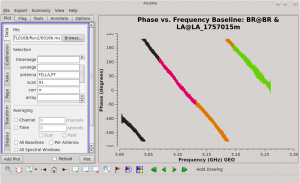
To determine which is the best to use as the reference antenna, use plotms to plot phase vs frequency for a single scan on a bright source (usually the fringe finder or bandpass calibrator). For this observation, use the third scan on 4C39.25, which is scan 91 from the listobs output. Inspect each of the 4 central antennas and use the one which has the most well-behaved phases. We start with scan 91 because it is near the middle of our observation, so 4C39.25 should be at relatively high elevations at all stations during that scan.
NOTE: For our observation, we know that it was windy at KP so we probably do not want to use that one as the reference antenna.
#In CASA
plotms(vis='tl016b.ms', xaxis='frequency', yaxis='phase', field='4C39.25', scan='91', correlation='ll', antenna='FD,LA,PT', iteraxis='baseline', coloraxis='spw')
Use the GUI to step though the baselines. Look at each antenna and look at both right- and left-hand polarization (correlation='rr' and correlation='ll' ). Our observation does not include the cross-hand polarizations (lr and rl), and you usually won't worry about inspecting them anyway since they will usually be too low to see anything useful.
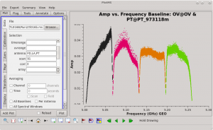
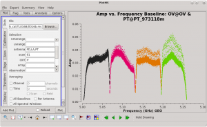
In the GUI, go to the "Axes" tab and change the "Data" axis to "Amp" (this is equivalent to settining yaxis='amplitude') to inspect the shapes of the bandpasses and look for RFI. If an antenna has strong RFI, you should not use it as the reference antenna.
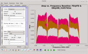
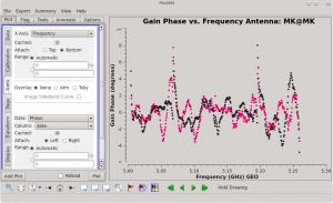
For this observation, we will use Fort Davis (FD) as the reference antenna. Its phases are fairly smooth, it is free of RFI, and the bandpasses look pretty clean (especially compared to PT in spw 2 and 3).
Identifying a Good Time Range for the Instrumental Delay Calibration
Next, we will look for a good time interval (about 1 minute long) for the instrumental delay calibration. This will be done using the fringe finder (4C39.25), so we should inspect each scan on it: 1, 44, 91, 134, and 181. We will want to plot amplitude vs time for each of these scans. To save time, we will just plot the baselines to the reference antenna, FD. Start by plotting scan 1.
#In CASA
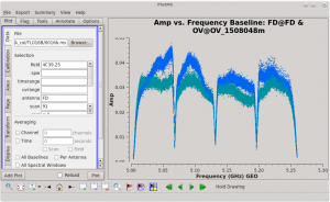
plotms(vis='tl016b.ms', xaxis='frequency', yaxis='amp', field='4C39.25', antenna='FD', scan='1', correlation='rr,ll', iteraxis='baseline', coloraxis='corr')
Use the GUI to step through each baseline for the scan. Then, use the "scan" field in the GUI to look at the other scans on 4C39.25 (scans 44, 91, 134, and 181). Look for outliers in the amplitude data. We want to use a time range with no RFI and with all antennas on source.
Notice that Saint Croix (SC) did not observe during scans 134 and 181, so we do not want to use either of those.
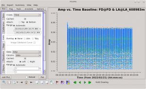
Scan 91 is close to the middle of the observation, and looks mostly clean. Use the plotms GUI to set the "scan" to "91" (in the "Data" tab) and the "X Axis" to "Time" (in the "Axes" tab) and step through the baselines again. Notice that some baselines have some higher amplitude points early on in this scan. We will want to avoid these early times. The time range 09:17:00 to 09:18:00 looks nice for each baseline to the reference antenna, so we will use that for our instrumental delay calibration later.
Flagging Data
Quack
VLBA observations often include a little bit of bad data at the beginnings of the scans, and sometimes at the ends of scans. An easy way to deal with this is to "quack" the data. Quacking is a completely optional step, and you should only do it if you see evidence for bad data at the beginnings or ends of scan. While inspecting our data previously, looking for a good reference antenna and time interval for the instrumental delay, we noticed that the beginnings of some scans had some higher amplitude points. So, we will want to quack this observation.
In CASA, you can quack your data using the flagdata task and setting mode='quack'. The amount of data to be flagged is controlled by the quackinterval parameter, which sets the time interval in seconds.
To flag the first 4 seconds of each scan:
#In CASA
flagdata(vis='tl016b.ms', mode='quack', quackinterval=4.0, quackmode='beg', quackincrement=True)
To flag the last 4 seconds of each scan:
#In CASA
flagdata(vis='tl016b.ms', mode='quack', quackinterval=4.0, quackmode='endb', quackincrement=True)
Historical Aside: There is some uncertainty about the origins of the term "quack". Most people assume it is some kind of reference to a duck. However, discussions with people who were working at NRAO in the late 1970s indicate it has nothing to do with waterfowl. Instead, "quack" refers to an unscrupulous/incompetent physician who treats the symptoms of a disease without treating the disease itself. In the early days of the VLA, the beginnings of scans often contained bad data. Several highly intelligent people spent many hours attempting to track down the cause of these issues, but nobody had any luck. Eventually, the decision was made to move on and simply get rid of the bad data. So, the original QUACK routine was written for the VLA DEC-10 computer to flag the beginnings of scans; it treated the symptoms (flagged the bad data) but did not do the hard work of curing the patient (fixing whatever was causing the bad data in the first place).
Automated Flagging
The the flagdata task includes a useful automated flagging mode known as "TFCrop". For more details on using the automated TFcrop mode, see the VLA CASA Flagging topical tutorial.
To begin, you just want to get a feel for what TFCrop will do to the data, which means you should set action='calculate' .
#In CASA
flagdata(vis='tl016b.ms', mode='tfcrop', datacolumn='data', timecutoff=4.0, freqcutoff=3.0, action='calculate', display='both')
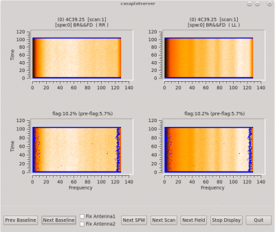
This will open a new window with a GUI. The top row of the GUI will display the data as it currently is. The bottom row shows what the data will look like after the flags are applied (blue regions are flagged). Step through the antennas by clicking "Next Baseline". Step through the spectral windows by clicking "Next SPW". Step through at least a few scans by clicking "Next Scan".
Using the default cut-off values of timecutoff=4.0, freqcutoff=3.0, and flagdimension='freqtime' appears to make the flagger focus on mostly on the edge channels. We do not necessarily want to get rid of those just yet. To exit the GUI, click "Quit". We will change the way TFCrop looks for bad data by setting flagdimension='time' , which will only look for outliers along the time axis. This should be fine, since we did not see any strong evidence for persistent RFI in the frequency dimension. Take a look at how the automatic flagging will approach things now:
#In CASA
flagdata(vis='tl016b.ms', mode='tfcrop', datacolumn='data', timecutoff=4.0, flagdimension='time', action='calculate', display='both')
Step through the baselines, spectral windows, and scans again. Note that the program now leaves the edge channels alone, but it still occasionally finds some outliers in along the time axis. With timecutoff=4.0, it should really only flag those data points that are 4-times the standard deviation in the time dimension. This should be sufficient to remove the worst of the time-dependent RFI in our observation.
To generate the flags, we will need to run flagdata again with action='apply' .
#In CASA
flagdata(vis='tl016b.ms', mode='tfcrop', datacolumn='data', timecutoff=4.0, flagdimension='time', action='apply', display='both')
You should double check that the automatic flagging will behave as you expect. Once you are satisfied that the flagging will do what you want, click "Stop Display". The program will then look through the entire observation and apply the flags.
NOTE: You can always exit the TFCrop mode without applying any flags by clicking "Quit", even when you set action='apply' .
Flagging "By Hand"
As telescope arrays become larger and more complex, automated flagging will become the primary means of excluding bad data (just look at what ALMA does). However, the current VLBA is still small enough that inspecting and flagging data oneself is not too painful.
You can look for obvious bad data using plotms. Be aware that while you can flag data in plotms, a major drawback to using plotms to flag data is that it makes undoing flags very difficult. The preferred method of flagging by hand is to identify the bad data with plotms, and then generate the flags with flagdata. It is recommended to be somewhat careful with flagging early on in the calibration process and only flag those data points that are obviously bad.
To start with, let's plot the bandpasses for each baseline to FD for all 5 scans on 4C39.25.
#In CASA
plotms(vis='tl016b.ms', xaxis='frequency', yaxis='amp', field='4C39.25', antenna='FD', scan='', correlation='rr,ll', iteraxis='baseline', coloraxis='scan')
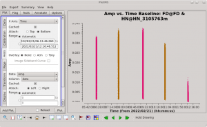
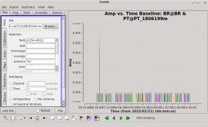
Using the GUI to step through the baselines, we can immediately see there is a problem with the FD-HN baseline for one scan. In the "Axes" tab of the GUI, switch the "X Axis" to "Time". Now we can see that the final scan on 4C39.25 at HN was much lower than the other scans. It's likely that the source was at very low elevation, so we should not trust those data. To make sure the problem was at HN, check that all baselines to HN have similar behavior; in the "Data" tab of the GUI, change "antenna" to "HN" and click "Plot". We can see that the final scan on 4C39.25 was low on all HN baselines. From our previous investigation of 4C39.25, we know that the final scan on this source was scan 181 (alternatively, you can either check the listobs output or use the "Locate" tool in plotms).
Flag all baselines to HN on the final scan of 4C39.25 using flagdata.
#In CASA
flagdata(vis='tl016b.ms', mode='manual', field='4C39.25', antenna='HN', scan='181')
If you kept your plotms window open, you can verify that the flagging has worked by checking the "Reload" box in the GUI and clicking "Plot" to re-plot the data. You should now see that the final scan on 4C39.25 is missing on all baselines to HN.
Next, let's take a look at the phase reference calibrator. To make sure 4C39.25 is the only source that got low at later times, we will start by plotting amplitude vs. time. We will use antenna='*&*' to plot only the cross-correlations.
#In CASA
plotms(vis='tl016b.ms', xaxis='time', yaxis='amp', field='J1154+6022', antenna='*&*', scan='', correlation='rr,ll', iteraxis='baseline', coloraxis='scan')
Note: You can plot just the autocorrelations by setting antenna='*&&&' , which can be a good way to look for RFI at a single station.
As you step through the baselines, you can see that J1154+6022 is fairly well-behaved. However, there are a few things that stand out. For example, there is a very hot time on the BR-PT baseline. Using the "Mark Regions" and "Locate" tools in the plotms, we can see that the problem is in scan 10. Using the GUI, we can take a closer look at scan 10; set antenna='BR&PT' , scan='10' , and spw='0' , then look at the other 3 spectral windows. There is obviously some bad data at the end of scan 10 in each spectral window. In fact, comparing scan 10 to other nearby scans (scan='6~14' ), it looks like all of scan 10 might be questionable. So, we will flag scan 10 on the BR-PT baseline using flagdata.
#In CASA
flagdata(vis='tl016b.ms', mode='manual', field='J1154+6022', antenna='BR&PT', scan='10')
Continuing to inspect the baselines, we can spot other problems. Again, use the "Mark Regions" and "Locate" buttons in plotms to identify the data that needs to be flagged, then use flagdata to create the flags.
#In CASA
flagdata(vis='tl016b.ms', mode='manual', field='J1154+6022', antenna='KP&LA', scan='221')
flagdata(vis='tl016b.ms', mode='manual', field='J1154+6022', antenna='LA&PT', scan='207')
flagdata(vis='tl016b.ms', mode='manual', field='J1154+6022', antenna='NL&PT', scan='213')
NOTE: You do not actually need to set mode='manual' when running flagdata via a task function call. The default setting for mode is already 'manual', so if you omit it from the command it will still automatically be set.
Now that we have flagged the calibrators, we should take a look at the science target. At this point, we should be careful about flagging too much on the science target because what initially looks like bad data may be poor calibration. However, obvious outliers can and should be flagged.
#In CASA
plotms(vis='tl016b.ms', xaxis='time', yaxis='amp', field='J1203+6031', antenna='*&*', scan='', correlation='rr,ll', iteraxis='baseline', coloraxis='scan')
Stepping through the baselines reveals some significant spikes in the data:
BR-OV scan 93
FD-HN scan 201
FD-LA scan 17
HN-KP scan 218
HN-LA scan 216
HN-NL scan 214
HN-PT scan 216
KP-NL scan 222
LA-NL scan 220
LA-PT scan 212
LA-PT scan 214
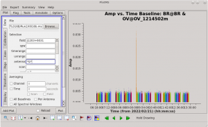
Because the scans on J1203+6031 are much longer than the scans on J1154+6022, we should take a closer look at the spikes and see if just a portion of the scan needs to be flagged. If you still have your plotms GUI open, go to the "Data" tab and set "Antenna" to "BR&OV" and "scan" to "93", and in the "Display" tab set "Colorize" to "Spw", then click "Plot". If you closed your plotms GUI, you can start it again using antenna='BR&OV' , scan='93' , coloraxis='spw'. You should see that the amplitude gets very large near the middle of the scan, but there is some kind of odd ringing behavior all throughout. It also appears that all of the spectral windows are affected. We should just flag the entire scan.
#In CASA
flagdata(vis='tl016b.ms', mode='manual', field='J1203+6031', antenna='BR&OV', scan='93')
Now, take a look at the FD-HN baseline on scan 201. You should see that the problem here is limited to roughly the last third of the scan. We will try keeping the first two-thirds, for now.
#In CASA
flagdata(vis='tl016b.ms', mode='manual', field='J1203+6031', antenna='FD&HN', scan='201', timerange='12:47:15~12:47:57')
Taking some time to look over the other problematic spots we identified above leads to the following flags:
#In CASA
flagdata(vis='tl016b.ms', mode='manual', field='J1203+6031', antenna='FD&LA', scan='17')
flagdata(vis='tl016b.ms', mode='manual', field='J1203+6031', antenna='HN&KP', scan='218', timerange='13:19:02~13:20:10')
flagdata(vis='tl016b.ms', mode='manual', field='J1203+6031', antenna='HN&LA', scan='216', timerange='13:16:46~13:17:10')
flagdata(vis='tl016b.ms', mode='manual', field='J1203+6031', antenna='HN&NL', scan='214', timerange='13:12:58~13:13:46')
flagdata(vis='tl016b.ms', mode='manual', field='J1203+6031', antenna='HN&PT', scan='216', timerange='13:16:24~13:17:10')
flagdata(vis='tl016b.ms', mode='manual', field='J1203+6031', antenna='KP&NL', scan='222', timerange='13:24:41~13:25:09')
flagdata(vis='tl016b.ms', mode='manual', field='J1203+6031', antenna='LA&NL', scan='220', timerange='13:21:31~13:21:59')
flagdata(vis='tl016b.ms', mode='manual', field='J1203+6031', antenna='LA&PT', scan='212,214')
The data should be pretty clean at this point, but we will need to keep an eye on things as we continue the calibration.
Calibrating the Data
Amplitude Corrections from Autocorrelations
Determine the amplitude corrections from the autocorrelations with accor.
#In CASA
accor(vis='tl016b.ms', caltable='tl016b.accor', solint='30s')
NOTE: This step is not required for EVN data, because the EVN correlator performs it during correlation.
Inspect the tl016b.accor solution table with plotms.
#In CASA
plotms(vis='tl016b.accor', xaxis='time', yaxis='amp', iteraxis='antenna', coloraxis='spw')
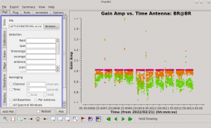
Ideally, all of the solutions should be very close to 1.0. Stepping through the antennas, it is clear that pretty much every station has significant outliers.
The AIPS VLBA utility script VLBACCOR smooths the autocorrelation corrections by default (with a smoothing time of 30 minutes). It is possible to do this smoothing in CASA 6.3 and later using the smoothcal task. Based on what we saw in our plotting, these data would likely benefit from some smoothing.
#In CASA
smoothcal(vis='tl016b.ms', tablein='tl016b.accor', caltable='tl016b_smooth.accor', smoothtype='median', smoothtime=1800.0)
Remember to check the smoothed solutions with plotms to make sure it was an improvement.
#In CASA
plotms(vis='tl016b_smooth.accor', xaxis='time', yaxis='amp', iteraxis='antenna', coloraxis='spw')
Things look better, but there are still some areas we will need to keep an eye on. Brewster (BR), Los Alamos (LA), and Saint Croix (SC) all have significant structure at later times, especially at the higher frequencies (spw's 2 and 3). Surprisingly, Kitt Peak (KP) looks very nice, even though we know it was windy at that station for at least a portion of the observation.
A Priori Calibration
Unlike the VLA, the VLBA cannot rely on bootstrapping absolute flux density calibration from a well-modeled calibrator. Instead, the VLBA relies on a combination of the system temperature and the known gain curve of the antennas (how the gain of the antenna changes with elevation). Both the system temperatures and gain curves are included in the FITS-IDI file, and both are imported into the Measurement Set with importfitsidi. To get the system temperature and gain curve information into a form that CASA can use for calibration, we use the gencal task to generate calibration tables.
System temperature:
gencal(vis='tl016b.ms', caltable='tl016b.tsys', caltype='tsys', uniform=False)
You will see several messages appear informing you that the Tsys values for many times were negative and will be flagged. Notice that the antenna associated with these bad Tsys values is "antenna id=0", which is Brewster (BR). Also, all of the bad Tsys values are in spw 2 and 3. From our plotting of the accor values, we knew that BR likely had issues in spw's 2 and 3.
Check the system temperature table with plotms.
#In CASA
plotms(vis='tl016b.tsys', xaxis='time', yaxis='tsys', iteraxis='antenna', coloraxis='spw')
Make sure to also plot the solutions with xaxis='freq' .
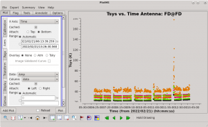
You should see that the remaining Tsys values for BR in spw 2 and 3 are pretty terrible. Also, KP spw 3, LA spw 2, NL spw 3, and SC spw 3 are a bit gross. Our chosen reference antenna, FD, looks pretty good except for one spike.
Notice that many of the minor "outlier" points are scans on the fringe finder 4C39.25. In most cases, including that apparent spike on FD, the 4C39.25 outlier points are the last scan on the source (scan 181). This could mean the source was simply at a very low elevation at most stations. We will need to be careful as we continue with the calibration to not use that last scan on 4C39.25 because it could introduce errors into our calibration. To be safe, we will flag that scan.
#In CASA
flagdata(vis='tl016b.ms', mode='manual', field='4C39.25', scan='181')
At this point, it is good to remind ourselves of the radio astronomer's credo: "With great power comes great responsibility." No, wait! The other one: "Bad data is worse than no data." With that in mind, we will flag the data in the measurement set corresponding to the really bad Tsys values. Just as we did in the Flagging "By Hand" section, we will fist identify the bad data using the "Mark Regions" and "Locate" tools in plotms, and create the flags using flagdata
#In CASA
flagdata(vis='tl016b.ms', mode='manual', antenna='BR', spw='2,3')
flagdata(vis='tl016b.ms', mode='manual', antenna='KP', spw='3')
flagdata(vis='tl016b.ms', mode='manual', antenna='LA', spw='2')
flagdata(vis='tl016b.ms', mode='manual', antenna='NL', spw='3')
flagdata(vis='tl016b.ms', mode='manual', antenna='SC', spw='3', scan='135~223')
Gain curve:
#In CASA
gencal(vis='tl016b.ms', caltable='tl016b.gcal', caltype='gc')
For this observation at 5 GHz, the gain curve is not very interesting, so we will not bother looking at the solutions now (although you can if you really want to). If your observation is at 12 GHz or higher, you will probably want to inspect the gain curve table with plotms.
NOTE: For EVN observations, the system temperatures and gain curves are provided in ANTAB files rather than in the FITS-IDI file. If you are working with EVN data, you must append the system temperature data to the FITS-IDI file before running importfitsidi. EVN gain curves must also be extracted from the ANTAB file. For more information, see the EVN Data Reduction Guide.
Instrumental Delay Calibration
Solve for the instrumental delays by using fringefit on a bright source (the "fringe finder"). In our case, the fringe finder is 4C39.25. Set the timerange to the one-minute time span you identified while inspecting the data earlier. Because we are only solving for the instrumental delays (changes in phase as a function of frequency), we will set zerorates=True to set all of the delay-rates (changes in phase as a function of time) to be zero.
#In CASA
fringefit(vis='tl016b.ms', caltable='tl016b.sbd', field='4C39.25', timerange='09:17:00~09:18:00', solint='inf', zerorates=True, refant='FD', minsnr=10, gaintable=['tl016b_smooth.accor', 'tl016b.gcal', 'tl016b.tsys'], interp=['nearest', 'nearest', 'nearest,nearest'], parang=True)
Watch the logger for any reports of low SNR and failures to converge on a solution. Ideally, the SNR for each station should be very high (for our data, all reported SNR values are larger than 3900, which is very good).
Once fringefit has finished, you should see the following in the logger:
Finished solving.
Calibration solve statistics per spw:  (expected/attempted/succeeded):
  Spw 0: 1/1/1
  Spw 1: 1/1/1
  Spw 2: 1/1/1
  Spw 3: 1/1/1
This is exactly what we expect to see. We are only attempting to get one solution per spw because we are only solving over a single solution interval (one minute of data from a single scan).
Apply the instrumental delay corrections using applycal.
#In CASA
applycal(vis='tl016b.ms', gaintable=['tl016b_smooth.accor', 'tl016b.gcal', 'tl016b.tsys', 'tl016b.sbd'], interp=['nearest', 'nearest', 'nearest,nearest', 'nearest'], parang=True)
NOTE: In applycal, the order in which you specify the list for gaintable sets the order for both interp and spwmap. If you change the order of gaintable, be sure to also change the order of interp and spwmap! Also, if you smoothed any of the solutions, be sure to use the appropriate filename for the smoothed table.
It may take a little while (~2 minutes or more) for applycal to finish. If you are watching the logger carefully, you will see the message "Adding CORRECTED_DATA column(s)". Because this is the first time that we have run applycal, CASA needs to create a new column containing the data with the corrections applied.
Check that applying the solutions resulted in improvements:
#In CASA
plotms(vis='tl016b.ms', field='4C39.25', xaxis='frequency', yaxis='phase', ydatacolumn='corrected', timerange='09:17:00~09:18:00', correlation='rr,ll', antenna='*&*', iteraxis='antenna', coloraxis='antenna2')
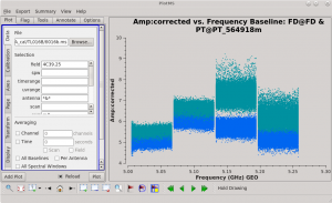
All of the phase values should now be clustered around 0 degrees. There may be some outliers near the band edges, especially on MK. This is nothing to worry about, yet.
Global Fringe Fitting
Now, we will solve for the time and frequency-dependent effects in phase using fringefit, also known as "global fringe fitting" (or sometimes "multi-band delay", if you combine all of the bands). We will need to pick a solution interval that is appropriate for our data. It should be at least 10 seconds, and no longer than the scan length on the phase reference calibrator. For this observation, we will use 30 seconds which will give us one solution per scan on the phase reference calibrator, and 7 solutions per scan on the fringe finder.
For refant, enter a list of antennas to try as the reference antenna. The preferred refant should be listed first, followed by the second choice, then third choice, and so on. It is not recommended to include Mauna Kea (MK) or Saint Croix (SC) in the list, unless the phase reference calibrator is very bright on the longest baselines. For our observation, BR had some serious issues in two of our four spectral windows, so we will omit it from our list of possible reference antennas, too. Set field to the fringe finder and phase reference calibrator.
#In CASA
fringefit(vis='tl016b.ms', caltable='tl016b.mbd', field='4C39.25, J1154+6022', solint='30s', minsnr=5, zerorates=False, refant='FD,PT,LA,KP,OV,NL,HN', gaintable=['tl016b_smooth.accor', 'tl016b.gcal', 'tl016b.tsys', 'tl016b.sbd'], interp=['nearest', 'nearest', 'nearest,nearest', 'nearest'], parang=True)
This step may take quite a while (probably at least 20 minutes), so this is a good opportunity to stand up, stretch, and go get a tasty beverage.
When the fringefit task is done, check the logger for the solution statistics ("expected/attempted/succeeded"). You want all three numbers to be the same, or at least very similar.
For our project, you should see something like this in the logger:
Finished solving.
Calibration solve statistics per spw:  (expected/attempted/succeeded):
  Spw 0: 263/256/256
  Spw 1: 263/256/256
  Spw 2: 263/256/256
  Spw 3: 263/256/256
For each spw, the "expected/attempted/succeeded" numbers are 263/256/256. Taking a closer look in the logger, you can find that the total number of solution intervals was 1052, and there were good solutions on 1024 intervals. In the CASA window itself, you may see several messages about "no unflagged data". Inspecting further, you can discover that all of these missing solutions are on scan 181, the final scan on 4C39.25 which we flagged back in the System Temperature step. So, these missing solutions are expected and we should continue with our calibration.
You should also look through the log for instances when the SNR was below your threshold (minsnr) and times when it took many iterations to get a good fit. If you see several cases of one or both of these, you may need to try longer solution intervals to get the global fringe fit to work optimally. Our data looks pretty good, though. There are a few cases where antenna 9 (SC) has low SNR late in the observation when the source would have been at low elevation, so these are to be expected.
Because fringefit ran successfully and we are satisfied that the number of solutions is appropriate, we should now take a look at the solutions with plotms.
#In CASA
plotms(vis='tl016b.mbd', xaxis='time', yaxis='phase', iteraxis='antenna', coloraxis='spw')
Use the GUI to switch the yaxis between 'phase', 'delay', and 'delayrate'. The phase and delay solutions should both vary smoothly with time. If they do not, you may need to smooth the table before applying it. The delay-rates should be clustered around zero with some scatter. You should see that the solutions on all antennas look very good.
Now that we are confident that the global/multi-band solutions are good, we will apply them with applycal.
#In CASA
applycal(vis='tl016b.ms', gaintable=['tl016b_smooth.accor', 'tl016b.gcal', 'tl016b.tsys', 'tl016b.sbd', 'tl016b.mbd'], interp=['nearest', 'nearest', 'nearest,nearest', 'nearest', 'linear'], parang=True)
It will probably take a while (about 3 minutes or longer) for applycal to run this time.
Take a look at the calibrated data with plotms to make sure the corrections are improving the phases.
#In CASA
plotms(vis='tl016b.ms', xaxis='frequency', yaxis='phase', ydatacolumn='data', field='4C39.25', antenna='*&*', scan='44', correlation='rr,ll', iteraxis='antenna', coloraxis='corr')
Use the GUI to step through the antennas. The uncalibrated data is pretty much a mess. Now, go to the "Axes" tab and change the Data Column from "data" to "corrected". The corrected data should look much better, with the phases centered around zero degrees with some scatter.
Bandpass Calibration
Now we will correct for the shape of the bandpass using the bandpass task. This step requires a very bright source (perferably >1 Jy on all baselines), so we will use our fringe finder 4C39.25. However, unlike when we solved for the instrumental delay (above), we will use all of the scans on the source.
#In CASA
bandpass(vis='tl016b.ms', caltable='tl016b.bpass', field='4C39.25', solint='inf', refant='FD', solnorm=True, bandtype='B', gaintable=['tl016b_smooth.accor', 'tl016b.gcal', 'tl016b.tsys', 'tl016b.sbd', 'tl016b.mbd'], interp=['nearest', 'nearest', 'nearest,nearest', 'nearest', 'linear'], parang=True)
Inspect the solutions with plotms.
#In CASA
plotms(vis='tl016b.bpass', xaxis='frequency', yaxis='amp', iteraxis='antenna', coloraxis='corr')
While looking over the solutions, also make sure to check the phases (uses the GUI to set yaxis='phase'). You should see that the phase solutions are all near zero.
Apply the solutions with applycal.
#In CASA
applycal(vis='tl016b.ms', gaintable=['tl016b_smooth.accor', 'tl016b.gcal', 'tl016b.tsys', 'tl016b.sbd', 'tl016b.mbd', 'tl016b.bpass'], interp=['nearest', 'nearest', 'nearest,nearest', 'nearest', 'linear', 'linear,linear'], parang=True)
It will probably take a while for applycal to run again, since you are also applying the solutions from the global fringe fitting.
After applying the bandpass solutions, take a look at the calibrated data with plotms.
#In CASA
plotms(vis='tl016b.ms', xaxis='frequency', yaxis='amp', ydatacolumn='corrected', field='4C39.25', antenna='*&*', correlation='rr,ll', iteraxis='baseline', coloraxis='corr')
The bands look pretty good, but there is some offset between the bands and between polarizations ("correlations") inside each band. This is usually not a big deal and can be corrected with self-calibration.
The bandpass calibration often does not perfectly calibrate the channels at the beginning and end of each spectral window. We can see such problems in our data where there are often outliers (both high and low) at the edges of each band. It is often a good idea to get rid of the edge channels that are not well-calibrated. We will use flagdata to get rid of some of the edge channels.
For our data, we will flag the first and last 3 channels of each spw.
#In CASA
flagdata(vis='tl016b.ms', spw='*:0~2;125~127')
Many experienced VLBA observers will not have any second thoughts about cutting out 8 or 12 channels on each side of the spw for continuum observations. If you start with flagging 3 channels on each side and think the amplitude vs frequency plots still look pretty gross, feel free to flag some more.
Final Amplitude Scaling and Flux Calibration
Any VLBA observation with wide bandwidths (256 MHz and larger), which is any observation done a bit rate of 2 Gbps or more, will require one extra calibration step at this point. The flux density scale for wideband VLBA observations can be off by up to 30% (although it usually only off by a few percent) if the calibration does not correctly account for the wide bandpasses. To do this, you need to run accor again after the bandpass calibration has been applied. The AIPS task that was developed to address this issue is called ACSCL. For more details on this topic, and how it was handled in AIPS, see VLBA Scientific Memo #37.
Our observation had 256 MHz of total bandwidth, so we should worry about this effect.
Prior to running accor this time, it is strongly recommended that users inspect the calibrated data and determine whether any channels will need to be excluded from imaging or other post-processing. Edge channels may need to be excluded if the bandpass calibration did not properly correct the band at the edges. From VLBA Scientific Memo #37, the standard recommendation is to use the inner ~75% of channels for PFB observations and the inner ~89% of channels for DDC observations. Any channels that are suspected to contain RFI should also be excluded. The actual channels used will depend on the individual observation and science goals.
We have already flagged the worst of the edge channels in the previous section. Inspecting the data after flagging reveals that the bands are fairly flat, but there may still be some small issues at the edges. Just to be safe, we will do the final re-scaling of the auto-correlation amplitudes with accor using the spectral channels 7 to 121.
NOTE: DO NOT APPLY THE SYSTEM TEMPERATURE OR GAIN CURVE TABLES WHEN DERIVING THESE SOLUTIONS.
#In CASA
accor(vis='tl016b.ms', spw='*:7~121', caltable='tl016b.acscl', solint='2min', gaintable=['tl016b_smooth.accor', 'tl016b.sbd', 'tl016b.mbd', 'tl016b.bpass'], interp=['nearest', 'nearest', 'linear', 'linear,linear'])
Check that the new accor solutions are also near 1.0 by plotting them with plotms.
#In CASA
plotms(vis='tl016b.acscl', xaxis='time', yaxis='amp', iteraxis='antenna', coloraxis='spw')
The AIPS VLBA utility script VLBAAMP smooths the autcorrelation corrections by default in exactly the same way as VLBACCOR. We will replicate the AIPS method by using the smoothcal task to smooth our .acscl table.
#In CASA
smoothcal(vis='tl016b.ms', tablein='tl016b.acscl', caltable='tl016b_smooth.acscl', smoothtype='median', smoothtime=1800.0)
Apply the final amplitude solutions with applycal. You should apply the system temperature and gain curve tables in this step.
#In CASA
applycal(vis='tl016b.ms', field='', gaintable=['tl016b_smooth.accor', 'tl016b.gcal', 'tl016b.tsys', 'tl016b.sbd', 'tl016b.mbd', 'tl016b.bpass', 'tl016b_smooth.acscl'], interp=['nearest', 'nearest', 'nearest,nearest', 'nearest', 'linear', 'linear,linear', 'nearest'], parang=True)
Congratulations! The data should be mostly calibrated at this point. At the very least, you should be able to make images of the calibrators.
Split Out Calibrated Data
It is generally recommended to split the measurement set after the initial calibration is complete. If you have multiple science targets, you should create a new MS for each science target + phase reference calibrator pair by setting the field paremeter to the appropriate values. Even if your observation only involved a single target, it is a good idea to split the MS once the initial calibration is complete. This will preserve the initially-calibrated data in case you make a mistake in any of the next steps and need to start over. Think of it as a "save point" in a video game (do you really want to have to go back to the beginning of the game when you could just start from the beginning of the current level?).
Split the calibrated MS using split.
#In CASA
split(vis='tl016b.ms', outputvis='tl016b_cal1.ms', field='J1154+6022,J1203+6031', spw='*:7~121', antenna='*&*', datacolumn='corrected')
You can name the new MS whatever you want, but using a naming scheme that keeps track of where it was in the calibration process will make your life easier if you make mistakes down the line. For this tutorial, we will use "tl016b_cal1.ms" to indicate it is where we ended up after the first calibration steps. Setting antenna='*&*' will leave the autocorrelations out of our new MS (we don't need them anymore). We should not need 4C39.25 for any of the next steps, so we will not bother to keep that source in our new MS. Also, note that we have selected only the spectral channels that we used during the final amplitude scaling step.
Self-Calibration of Phase Reference Calibrator
Despite our best efforts with the initial calibration, VLBA observations will almost always require additional steps to improve the calibration. Because the VLBA antennas are separated by such large distances, the phases may not be perfectly calibrated by fringe fitting alone. This is partly because each antenna may be looking through vastly different troposphere/ionosphere, and partly because the phase reference calibrators are rarely point sources on long baselines (and fringe-fitting usually assumes the calibrators are point sources on all baselines).
We will improve the calibration using "self-calibration". The process of self-calibration involves building models of the sources, refining the calibration based on those models, and then repeating until you converge to a good solution. The models are created during the imaging process. Each iteration of self-calibration should produce images with lower noise.
Each time the noise is reduced, you may notice dimmer structures appear. This is where you need to be careful. Including an apparent structure in a model for self-calibration can "build in" features that are not real. A good rule of thumb is "if you can't self-calibrate a structure away, it is probably real". So, if you are uncertain whether a newly apparent component is real or not, first try to self-calibrate without including that component in the model. If it sticks around, it is probably a real structure and including it in the next model should further improve the calibration and lower the noise in the next image.
The first step in phase self-calibration is to create an image/model of a source, usually the phase reference calibrator. Fringe finders and bandpass calibrators are easy to self-calibrate (because they are so bright), but they are usually only observed a few times throughout the observation so any solutions derived from self-calibrating on them will not have a large impact on the overall calibration of your science target.
Imaging the Calibrator
To create images of our sources, we will use tclean.
In order to make an image of our phase reference calibrator (J1154+6022), we will first need to determine a few imaging parameters.
First, we need to know the "cell size" to use. The cell size is angular dimension of the image pixels (e.g., 1 arcsecond by 1 arcsecond). In tclean, the cell size is specified with the parameter cell. The formula to estimate the appropriate value for cell is:
[math]\displaystyle{ cell \approx \frac{206265}{N_{s} D_{max}[\lambda]} arcseconds }[/math]
where [math]\displaystyle{ N_{s} }[/math] is the Nyquist sampling factor, and [math]\displaystyle{ D_{max}[\lambda] }[/math] is the longest baseline in units of the observed wavelength.
For VLBI imaging, you typically want the [math]\displaystyle{ N_{s} }[/math] to be about 5 or 6. You can calculate the value of [math]\displaystyle{ D_{max}[\lambda] }[/math] on your own, or you can just plot the data using plotms and set xaxis='uvwave' . We will limit the amount of data we need to plot by only plotting the longest baseline: MK-SC.
#In CASA
plotms(vis='tl016b_cal1.ms', xaxis='uvwave', yaxis='amp', field='J1154+6022', antenna='MK&SC', correlation='rr,ll')
You should find that the maximum baseline is about 151 megawavelengths ([math]\displaystyle{ 1.51 \times 10^{8} }[/math] wavelengths). Using [math]\displaystyle{ N_{s}=6 }[/math], we estimate that our cell size should be about 0.000228 arcseconds (or 0.228 milliarcseconds). However, our formula for estimating the cell size assumes that the restoring beam has a Gaussian shape, which is not often true for VLBI observations. It is usually a good idea to use a slightly smaller cell size than the formula estimates. For our images, we will use cell='0.2mas' .
Now that we have our cell size, the next parameter we need to determine is the image size (imsize). Many programs (like difmap and AIPS) require that the image size be a power of 2 (256, 512, 1024, etc.). CASA does not have this requirement, but it is recommended that the image size be even and factorizable by 2, 3, and 5 only. In other words, set imsize[math]\displaystyle{ =2^{i}\times3^{j}\times5^{k} }[/math], where [math]\displaystyle{ i }[/math], [math]\displaystyle{ j }[/math], and [math]\displaystyle{ k }[/math] are positive integers (including 0). A good rule of thumb is to start with a power of 2 and then multiply by 10. So, sizes like 320, 640, 1280, etc. would all work well. For most phase reference calibrators, an image size of 640 should be fine. (You can always change it, if you need a bigger or smaller image.)
NOTE: If you know your preferred image size and want to use the closest optimal imsize, you can use the process described in the tclean imsize parameter documentation to determine what imsize to use.
The next two parameters to choose are relatively straightforward for us. For VLBA continuum observations, you will usually want to use pure natural weighting (weighting='natural' ). Because we are just making a continuum image, we will use stokes='I' to make a total intensity map.
The final parameter to choose is the deconvolver. In order to decide which deconvolver to use, you will need to calculate the fractional bandwidth of the observation. The fractional bandwidth is the total per-polarization bandwidth divided by the center frequency. The total per-polarization bandwidth for our observation is 256 MHz and our center frequency is 5132 MHz, so our fractional bandwidth is ~0.04. Because our fractional bandwidth is less than 0.1, we can use the clark or hogbom deconvolver. We will go with deconvolver='clark' for our observation. If the fractional bandwidth was about 0.1 or larger, we would probably want to use the multi-term, multi-frequency synthesis deconvolver (mtmfs).
NOTE: If a source is compact (point-like) and the fractional bandwidth is ~0.1, you probably will not see any major differences between the hogbom, clark, and mtmfs deconvolvers. However, if the source is extended or complex (e.g., has a long jet) and/or the fractional bandwidth is >0.2 (e.g., two widely-spaced sidebands that you are imaging together), the mtmfs deconvolver will produce vastly superior images. A guide to using tclean with the mtmfs deconvolver can be found in the VLA Imaging CASA Guide.
#In CASA
tclean(vis='tl016b_cal1.ms', field='J1154+6022', imagename='J1154_sc1', imsize=[640], cell=['0.2mas'], stokes='I', deconvolver='clark', weighting='natural', niter=1000, interactive=True, savemodel='modelcolumn')
Setting interactive=True will allow us to define the areas where there is real flux from the source ("clean windows"). The value for niter needs to be large enough that we can go through enough clean iterations to recover most of the source flux. You can set niter to any arbitrarily large number (a few hundred should be plenty), but 1000 is an easy value to remember. Setting savemodel='modelcolumn' will save the model we create for the image to the model column of the measurement set so we can use it for self-calibration.
Running tclean with interactive=True will open a new Viewer Display Panel where you can control the cleaning of the image. You should see that J1154+6022 is fairly point-like. Use the zoom tool to select the region around the source. Use the "polygon drawing" tool to draw a clean window around the source, excluding the stuff to the left and right of the bright source. Click on the "Continue deconvolution" button (the green circular arrow on the right). Check the residuals when the display updates. Stop cleaning when the area around the source looks noise-like. For example, if you notice positive and negative regions with similar magnitudes (e.g., +0.003 and -0.003) inside your clean window, that is probably a good time to stop cleaning. To stop the cleaning process, click the "stop deconvolving now" button (the red circle with the white "X"). It may take tclean a while to finish and close.
NOTE: If you need to delete a clean window, select "Erase" at the far left of the green region in the GUI and draw a box around the clean window(s) you want to delete, then double click. Remember to select "Add" again to define new clean windows.
The tclean task will make several output files, all named with the prefix given as imagename. These include:
- .image: final restored image, with the clean components convolved with a restoring beam and added to the remaining residuals at the end of the imaging process
- .pb: effective response of the telescope (the primary beam)
- .mask: areas where tclean has been allowed to search for emission
- .model: sum of all the clean components, which also has been stored as the MODEL_DATA column in the measurement set if you set savemodel='modelcolumn'
- .psf: dirty beam, which is being deconvolved from the true sky brightness during the clean process
- .residual: what is left at the end of the deconvolution process; this is useful to diagnose whether or not to clean more deeply
- .sumwt: a single pixel image containing sum of weights per plane
NOTE: For some excellent illustrations of what is happening during the cleaning process, see the DARA EVN tutorial Part 2, Section 3A and Section 3D.
Tracking Improvement
To ensure that self-calibration is actually helping to improve the quality of the images, you should track some image statistics. The most reliable way to do this is to define 2 boxes in the image; one box that contains the source ("on-source"), and one box that does not contain any part of the source ("off-source"). You can use imview to inspect the image and determine where to place the on-source and off-source boxes.
#In CASA
imview
In the GUI, go to Data->Open->J1154_sc1.image, then click "raster image" to load the image we just created. Use the zoom tool to select the area around the source. Use the "rectangle drawing" tool to create a box around the source and record the pixel locations of the lower left and upper right corners. The on-source box should be fairly small and fit tightly around the source. For example, lower left = [305,303], upper right = [335,340] looks like it should work. Now, zoom out and draw another box somewhere off the source. You can make the off-source box pretty big. For example, lower left = [71,409], upper right = [588,604]. To make things a little easier, we will assign the values of our on- and off-source boxes to some variables in CASA:
#In CASA
j1154_onbox='305,303,335,340'
j1154_offbox='71,409,588,604'
Once you have your on- and off-source boxes defined, use the task imstat to gather some statistics about those regions.
#In CASA
imstat(imagename='J1154_sc1.image', box=j1154_onbox)
imstat(imagename='J1154_sc1.image', box=j1154_offbox)
Running imstat will return several values in both the logger and the CASA terminal. The values of interest for the self-calibration process are the on-source peak value ("max"), the on-source total flux density ("flux"), and the off-source RMS value ("rms"). It is a very good idea to record each of these values for each image (including the first image without any self-calibration applied) as you proceed with self-calibration. Ideally, the on-source peak and total flux values will increase slightly and the off-source RMS will decrease significantly as you improve the calibration. However, be very suspicious of large increases (>10%) in flux density values, especially when the off-source RMS does not improve dramatically.
For the first image of J1154+6022, the values should be fairly close to:
On-source:
'flux': 0.195
'max': 0.190
Off-source:
'rms': 0.00068
Record these values in your notes so you have a way to check if self-calibration is leading to improvements in the images.
Phase Self-Calibration
Now that we have an initial model of the phase reference calibrator (from the image), we can begin the self-calibration process. In CASA, this is done with the gaincal task.
First, we will refine the delays.
#In CASA
gaincal(vis='tl016b_cal1.ms', field='J1154+6022', caltable='tl016b_cal1.dcal', solint='inf', refant='FD', minblperant=3, gaintype='K', calmode='p', parang=False)
Just as when running fringefit, you should check the logger to see how well the calibration is working. In the logger output, you should see:
Finished solving.
Calibration solve statistics per spw:  (expected/attempted/succeeded):
  Spw 0: 114/114/114
  Spw 1: 114/114/114
  Spw 2: 114/114/114
  Spw 3: 114/114/114
Because all of the numbers match, we know that we have obtained good solutions for each spectral window and for each solution interval.
Inspect the delay solution table with plotms.
#In CASA
plotms(vis='tl016b_cal1.dcal', xaxis='time', yaxis='delay', iteraxis='antenna', coloraxis='spw')
All of the solutions should be near zero, with some small scatter.
Next, we will refine the phases. For this step, we will set the solution interval to 20 seconds (solint='20s' ) to give us two solutions per scan on the phase reference calibrator.
#In CASA
gaincal(vis='tl016b_cal1.ms', field='J1154+6022', caltable='tl016b_cal1.pcal', solint='20s', refant='FD', minblperant=3, gaintype='G', calmode='p', gaintable=['tl016b_cal1.dcal'], interp=['linear'], parang=False)
In the CASA window, you may see several "Found no unflagged data" messages. If you inspect the listobs output for the times specified, you will see that the scans with the errors were a little longer than 40 seconds and less than 60 seconds. Therefore, there are some "orphan" solution intervals (intervals shorter than the solution interval where solutions cannot be obtained) on these scans. This is nothing to worry about.
Checking the logger, you should see:
Finished solving.
Calibration solve statistics per spw:  (expected/attempted/succeeded):
  Spw 0: 266/238/238
  Spw 1: 266/238/238
  Spw 2: 266/238/238
  Spw 3: 266/238/238
While the numbers do not match, we know that cause of this and we are not worried about it.
Inspect the phase solution table with plotms.
#In CASA
plotms(vis='tl016b_cal1.pcal', xaxis='time', yaxis='phase', iteraxis='antenna', coloraxis='spw')
As with the delays, all of the solutions should be clustered around zero.
Notice that when refining both the delays and the phases we set minblperant=3 because closure phases require at least 3 baselines.
Apply the phase self-calibration solutions to the phase reference calibrator.
#In CASA
applycal(vis='tl016b_cal1.ms', field='J1154+6022', gaintable=['tl016b_cal1.dcal','tl016b_cal1.pcal'], interp=['linear','linear'], parang=False)
Make a new image after the improved phase calibration using tclean just as we did previously. Remember to use a new imagename for this new image of the phase self-calibrated data.
#In CASA
tclean(vis='tl016b_cal1.ms', field='J1154+6022', imagename='J1154_sc2', imsize=[640], cell=['0.2mas'], stokes='I', deconvolver='clark', weighting='natural', niter=1000, interactive=True, savemodel='modelcolumn')
Once you have created the new image, check for improvement with imstat. As long as you did not change the imsize or cell parameters, you can use the same on- and off-source boxes that we defined earlier.
#In CASA
imstat(imagename='J1154_sc2.image', box=j1154_onbox)
imstat(imagename='J1154_sc2.image', box=j1154_offbox)
For the second image of J1154+6022, the values should be fairly close to:
On-source:
'flux': 0.195
'max': 0.191
Off-source:
'rms': 0.00068
Record these values in your notes.
We did not see a great deal of improvement after applying the phase self-calibration. This is not uncommon for VLBA observations of phase reference calibrators in CASA. This may be partially due to the fact that we have already done fringe fitting on the phase reference calibrator, so our phase calibration is already pretty good. Also, the phase reference source for this observation is pretty close to being a point source, so there is really not much room for improvement in just the phases. We should see more dramatic improvement after applying the amplitude self-calibration in the next step.
Amplitude Self-Calibration
#In CASA
gaincal(vis='tl016b_cal1.ms', field='J1154+6022', caltable='tl016b_cal1.apcal', solint='inf', refant='FD', minblperant=4, gaintype='G', calmode='ap', solnorm=True, gaintable=['tl016b_cal1.dcal','tl016b_cal1.pcal'], interp=['linear','linear'], parang=False)
Notice that we have set minblperant=4 because closure amplitudes require 4 baselines, and solint='inf' to use the full scan for each solution.
In the logger, you should see:
Finished solving.
Calibration solve statistics per spw:  (expected/attempted/succeeded):
  Spw 0: 114/114/114
  Spw 1: 114/114/114
  Spw 2: 114/114/114
  Spw 3: 114/114/114
All of the numbers match, which is what we like to see.
Above the solution statistics in the logger, you should also see messages about the normilazation amplitudes.
Applying refant: FD refantmode = flex (hold alternate refants' phase constant) when refant flagged
Normalizing solution amplitudes per spw with MEAN
 Normalization factor (MEAN) for spw 0 = 1.0534
 Normalization factor (MEAN) for spw 1 = 1.10366
 Normalization factor (MEAN) for spw 2 = 1.0002
 Normalization factor (MEAN) for spw 3 = 0.995902
Writing solutions to table: tl016b_cal1.apcal
The mean normalization factors are all close to 1.0, which is what we expect since we set solnorm=True. If the mean values were far from 1.0, we would be worried that the amplitude self-calibration was not working properly (perhaps one or two of the antennas were drastically low or high).
We should also take a look at the solutions on each telescope using plotms.
#In CASA
plotms(vis='tl016b_cal1.apcal', xaxis='time', yaxis='amp', iteraxis='antenna', coloraxis='spw')
Most of the antennas look very good. The solutions on Los Alamos (LA) and North Liberty (NL) are a little worrying, but not so much that we shouldn't believe them.
Apply the amplitude solutions to the phase reference calibrator.
#In CASA
applycal(vis='tl016b_cal1.ms', field='J1154+6022', gaintable=['tl016b_cal1.dcal','tl016b_cal1.pcal','tl016b_cal1.apcal'], interp=['linear','linear','linear'], parang=False)
Make one last image of the phase reference calibrator, just to check for improvements. Since we will not be doing any more self-calibration on this source, we will set savemodel='none' to save some time and disk space. Remember to use a new imagename again.
#In CASA
tclean(vis='tl016b_cal1.ms', field='J1154+6022', imagename='J1154_sc3', imsize=[640], cell=['0.2mas'], stokes='I', deconvolver='clark', weighting='natural', niter=1000, interactive=True, savemodel='none')
Check the image statistics
#In CASA
imstat(imagename='J1154_sc3.image', box=j1154_onbox)
imstat(imagename='J1154_sc3.image', box=j1154_offbox)
For the final image of J1154+6022, the values should be fairly close to:
On-source:
'flux': 0.215
'max': 0.209
Off-source:
'rms': 0.00016
This is a significant improvement over the phase self-calibrated image!
Apply Calibration to Science Target
Up to this point, we have just been applying the self-calibration solutions to the phase reference calibrator. Now, we will apply the solutions to the science target.
#In CASA
applycal(vis='tl016b_cal1.ms', field='J1203+6031', gaintable=['tl016b_cal1.dcal','tl016b_cal1.pcal','tl016b_cal1.apcal'], interp=['linear','linear','linear'], applymode='calonly', parang=False)
Notice that we set applymode='calonly' to avoid doing any extra flagging on the science target.
Split Out Science Target
Now that the calibration of the science target has been improved thanks to self-calibration on the phase reference calibrator, we should split out the science target.
#In CASA
split(vis='tl016b_cal1.ms', outputvis='tl016b_cal2.ms', field='J1203+6031', datacolumn='corrected')
Image the Science Target
Now that we have a fully-calibrated science target, it is finally time to make an image of it.
#In CASA
tclean(vis='tl016b_cal2.ms', field='J1203+6031', imagename='J1203_im1', imsize=[640], cell=['0.2mas'], stokes='I', deconvolver='clark', weighting='natural', niter=1000, interactive=True, savemodel='modelcolumn')
Notice that we have set savemodel='modelcolumn' in case it is bright enough to self-calibrate (spoiler alert: it is).
Just as we did with the phase reference calibrator, we will zoom in on J1203+6031 and create a clean region using the "polygon drawing" tool. We see some symmetric "wings" around the source that we are not yet sure are real, so we will exclude those from our clean window. Click the "Continue deconvolution" button to begin the cleaning process.
After a couple iterations of cleaning, you should start to see structure appear to the south of the clean region. This is real! J1203+6031 has a jet that extends nearly due south of the core. Create a new clean region around this jet (and adjust your clean region around the core if it looks like you are missing some of the flux around there) and continue cleaning.
NOTE: If you are not sure about whether a structure in the residual image is real, do not put a clean region around it. You can always try cleaning around it to see if it goes away, or (if the source is bright enough) try to self-calibrate it away.
Stop cleaning when the residual image looks noise-like (it should take ~4 times clicking the "continue" button, total). It will take a while for tclean to finish because it will populate the model column of the measurement set.
Take a look at the image you have created with imview. Click on the "Open Data..." icon (the folder on the far left of the toolbar) to open the Data manager GUI. Look for the file "J1203_im1.image" and click on both "raster image" and "contour map". This should load the image in the viewer with the default settings. Click on the "Data Display Options" icon (the wrench on the far left) to open a GUI that will allow you to adjust how the image is displayed. You should see two tabs in the Data Display Options GUI: "J1203_im1.image-raster" and "J1203_im1.image". The "image-raster" tab has options for the colorscale image, and the "image" tab has options for the contour settings. Feel free to play with all of the settings to see what they do. When you are done playing, go to the "image-raster" tab and set "Data Range" to [0, 0.06], "Scaling Power Cycles" to -1.5, and "Color Map" to "Hot Metal 2". Next, go to the "image" tab and set "Base Contour Level" to 0.001, "Unit Contour Level" to 0.05, and "Relative Contour Levels" to [0.005, 0.01, 0.05, 0.1, 0.2, 0.4, 0.8]. Compare your image to the one shown below.
It is now left to the user to attempt to self-calibrate J1203+6031. It is not recommended to do amplitude self-calibration on this source (it is too dim). Remember to track the improvements by getting the image statistics from an on-source region and off-source region. You should refine the delays just once, but you should try an iterative process for refining the phases by starting with longer solutions intervals (start with solint='inf' ) and then using shorter solution intervals (solint='60s' , solint='30s' ). Remember to make a new image after each iteration of phase self-calibration.
As the calibration improves, you should see a longer and longer jet appear in the residual images. However, this also means your model is getting increasingly complicated and it will take longer and longer (~10 minutes or more) for tclean to write the model column after you are done cleaning.
After doing the final phase self-calibration with solint='30s' , make one last image (remember to set savemodel='none' for this image to save time and disk space!). The off-source rms in the final image should be close to 0.00014 Jy/beam, and the peak flux density in the core region should be about 0.083 Jy/beam. Take a look at the final image with imview and see if you can get it to match the example below (hint, use the "Rainbow 3" color map and try a lower base contour level than we used for the first image).
Congratulations! You have successfully calibrated a phase-referenced VLBA observation in CASA!

