VLA high frequency Spectral Line tutorial - IRC+10216-CASA6.5.3
This guide is for CASA version 6.5.3
This tutorial describes how to calibrate and image high-frequency (Ka Band) EVLA observations of two spectral lines toward the Asymptotic Giant Branch (AGB) star IRC+10216. For an introduction to using CASA, please see the Getting Started in CASA guide.
Note that for the purposes of this tutorial it is safe to ignore warning messages in CASA that the leap second table is out of date, although these can resolved by Updating the CASA Data Repository.
Scientific overview of IRC+10216
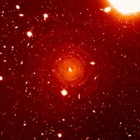
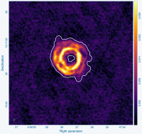
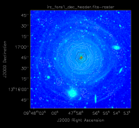
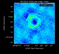
IRC+10216 (CW Leo, see Figure 1) is a 16th magnitude star in the optical, but the brightest star in the sky at a wavelength of 5 micrometer (60 THz). It was discovered during the first survey of the infrared sky, carried out by Bob Leighton and Gerry Neugebauer in 1965. This Asymptotic Giant Branch star is a Mira-type variable going through prodigious episodic mass loss. The dust condensed from the atmosphere during the mass loss is responsible for the millimeter and infrared emission; the radio continuum emission emerges from the stellar photosphere. Molecules form along with the dust, and a steady state chemistry occurs in the dense inner regions (Tsuji 1973 A&A 23, 411). As the density of the circumstellar material drops during the expansion of the outflow, the chemistry freezes while the molecules continue their long coast outward into the Galaxy. As the shell thins, ultraviolet light from the ambient Galactic radiation field penetrates the dust and initiates new chemistry in the gas.
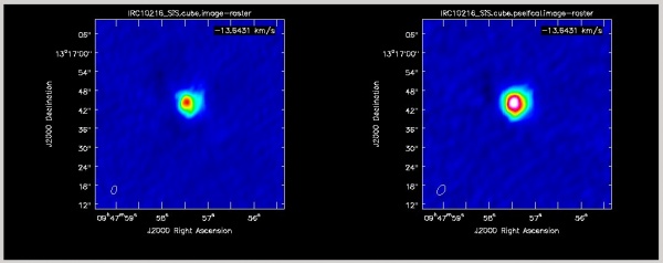
Silicon monosulfide (SiS) is a simple molecule created in the dense inner envelope chemistry and is photodissociated as it coasts out into the shell. It is observed as centrally concentrated emission in this tutorial. Interestingly, in the J=1-0 transition at 18.15 GHz, the SiS line shape is much different from what is seen here in the J=2-1 transition at 36.31 GHz. At the extreme velocities in the profile, very bright narrow emission is seen which has been interpreted as maser emission. More VLA observations of this line can be found in the NRAO Data Archive.
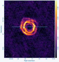
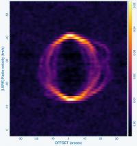
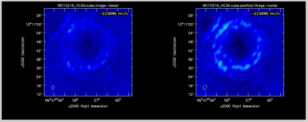
Cyanoacetylene (HC3N), a more complex molecule, is created by photochemistry that is triggered when atoms and pieces of molecules, destroyed by ultraviolet radiation, undergo the next phase of chemistry in the shell. In addition to its rotational modes, HC3N has many vibrational modes which may be excited. Owing to this, it can re-radiate energy absorbed from ultraviolet radiation more effectively than some molecules with a single bond. Eventually, it too is destroyed. However, during its brief existence, its rise to abundance in the envelope results in a ring of emission, which is what is observed in this VLA tutorial. Cordiner & Millar (2009, ApJ, 697, 68) describe a new chemical model for the shell, which also takes into account the variation of mass loss by the star. These authors show that in addition to purely chemical effects, local gas and dust density peaks play a role in shaping the observed emission.
Obtaining the data
In this 36 GHz VLA observation, two subbands with an 8 MHz bandwidth and 64 channels of 125 kHz (~1.0 km/s) spectral resolution were tuned to observe the SiS J=2-1 and HC3N J=4-3 lines. The first subband, targeting SiS, has a center frequency of 36.315 GHz and the second subband, targeting HC3N, has a center frequency at 36.398 GHz. In addition to these narrow-bandwidth subbands or "spectral windows" (sometimes abbreviated as spw in CASA) there are four subbands with 128 MHz bandwidth optimized for continuum sensitivity arranged between 36.5-37.0 GHz. These "continuum" subbands are not investigated in this tutorial but may be analyzed using the archive dataset by interested users.
To obtain the raw data for this project search the project code "TDRW0001" on the NRAO Science Archive and select the execution sb35770743.eb357744735.58429.44719293981 (file size 15.0 GB). To reduce the data file size and avoid computationally expensive conversion steps, we provide a minimally processed Measurement Set (MS) that may be downloaded from http://casa.nrao.edu/Data/EVLA/IRC10216/TDRW0001_10s.ms.tgz (file size 1.0 GB).
Once the download is complete, unzip and unpack the file by executing the following code in a shell or terminal:
tar -xzf TDRW0001_10s.tar.gz
These files were created by first converting the raw SDM-BDF data from the archive into an MS using the CASA task importasdm. So-called "online" flags were applied for known bad data using the flagdata task (i.e., using flag modes "quack", "shadow", and "clip"). The two spectral windows of interest, 2 and 3, were then sub-selected and the original 1 second visibility integrations were time averaged to 10 seconds using the task mstransform. The commands to reproduce these steps are included at the end of this tutorial in the section #All commands summarized.
The latter step produces a significantly smaller data set for processing in this tutorial, but leads to modest time-averaging amplitude losses for emission at the edge of the field. In practice, one should estimate the acceptable amplitude loss for the given science case, array configuration, and maximum baseline (see Time-Averaging Loss).
How to use this CASA guide
As mentioned above, please use CASA version 6.5.3 for this tutorial.
There are several ways to interact with CASA, described in more detail in Getting Started in CASA. In this tutorial we show how to use two different forms for interactive use and also include instructions on how the commands shown may be executed as a script. The interactive methods are intended to be used from the CASA shell or prompt. For completeness both interactive calling conventions are shown for some commands, please take care not to run same task with identical parameters twice.
- The first interactive method uses special CASA tasks to incrementally configure the parameters of CASA tasks and then execute them. This method is especially useful for repeatedly running the same command while only varying one or a few inputs. Using this method one types default taskname to load the task, inp to examine the inputs (see Figure 2), and go once those inputs have been set to your satisfaction. Inputs that have been modified from their default values are shown in blue. Default values are shown in the terminal's default foreground color (white on black in Fig. 2). Invalid inputs are shown in red and need to be fixed before a task can be run successfully with go. Input parameters are configured individually on the command line. For example, one could modify the selectdata parameter to False by typing selectdata=False<ENTER>. Once a task has been run, the set of inputs are stored and can be retrieved via tget taskname ; subsequent runs will overwrite the previous tget file. To reset a task to its default settings type, default taskname. An example using the task listobs is shown below:
# Interactive CASA
# Reset the input parameters for the task 'listobs'.
default listobs

# Print an overview to the terminal of how the task is configured.
# See Figure 2 for example output.
inp

# We set two input parameters below: one for the MS file name and
# another for the file name to store the output into.
vis = "data.ms"
listfile = "listobs_output.txt"

# We now run 'inp' again. It is best practice to always double-check
# the input parameters before running the task and to fix invalid
# parameter values shown in red.
inp

# Execute the task as configured.
go
- Disclaimer: CASA 6 has a bug when using inp taskname to switch to a new active task. If this method is used, then CASA will sometimes apply the global default parameters of the previous task to the current task in use. This can lead to using invalid global parameters. This guide uses default taskname to initialize the task, which will always apply the correct default parameters per task. We recommend using this method on your own as well until the CASA team is able to resolve the issue.
- The second interactive method uses standard Python function call syntax. While somewhat more verbose, this syntax simplifies the process of recording commands for later re-use in user-developed scripts or larger Python programs. In this case, all of the desired inputs to a task are provided at once on the CASA command line. This tutorial is made up of such calls, which were developed by looking at the inputs for each task and deciding what is needed to be changed from the default values. For task function calls, only parameters that you want to be different from their defaults need to be set. Using the same example as above for listobs:
# Python function call syntax.
# Type <ENTER> after the open-parenthesis to drop down a line.
# The close-parenthesis at the end is required to execute the function.
listobs(
    vis="data.ms",
    listfile="listobs_output.txt",
)
- Note that for both methods described above, the CASA shell is simply a specially configured Python interpreter, and thus all valid syntax for the Python programming language may be executed. This includes defining variables, using for loops, and declaring user-defined functions. CASA tasks are special purpose Python functions designed for specific data processing tasks. The CASA shell uses IPython to provide interactive features such as auto-completion of names, command history and search, and syntax highlighting. Detailed help on what a task does and what the input parameters do can be obtained for any task by typing help taskname. One can also search the CASA documentation on https://casadocs.readthedocs.io or call doc taskname from CASA to open the ReadTheDocs page automatically in the system's web-browser.
- Lastly, commands can be run non-interactively by executing a script. A series of task function calls can be combined together in a text file (script) along with other arbitrary Python statements, and run from within CASA via execfile('scriptname.py'). This and other CASA Tutorial Guides have been designed to be extracted into a script via the script extractor by using the method described within the Extracting scripts from these tutorials page. Should you use the script generated by the script extractor for this CASA Guide, be aware that it will require some small amount of interaction related to the plotting, occasionally suggesting that you close the graphics window and hitting return in the terminal to proceed. It is in fact unnecessary to close the graphics windows (it is suggested that you do so purely to keep your desktop uncluttered).
Initial inspection and overview
Observing logs
The VLA operator keeps an observing log for all observations, and these logs frequently contain pertinent information, such as poorly performing antennas or periods of high-wind or cloud cover. To access the operator logs for this dataset, go to the observing log website and enter a date range covering 7 November 2018. Click the "Show logs" button and on the following page select the project "TDRW0001" to download the log as a PDF file. Information of interest from this observation is repeated below:
INFORMATION FROM OBSERVING LOG:
Top left:
  Date of the observation: 07-Nov-2018
  Antenna configuration is "D"
  Antenna 26 (ea26) is undergoing routine maintenance and not included in the observations
Remarks on weather conditions:
  Sky is clear and low winds (1-2 m/s) throughout the observing period.
Operator comments:
  Antenna 27 (ea27) has recently been moved and has updated location data.
  Antenna 14 (ea14) the Front End team has begun warming the X Band receiver in order to replace it,
                    and the sensitivity is limited as a result. The X Band receiver is used for
                    antenna pointing calibration and the Ka Band for the science goals, thus this
                    and the next issue may affect the pointing accuracy of this antenna.
  Antenna 14 (ea14) the LO-IF team reports that the IF B is dead when moving into X Band.
  Antenna  1 (ea01) the Servo team reports a failure in the azimuth encoder, resulting in the
                    loss of about 3.6 minutes of data (see the right-most column).
All of the logged information should be kept in mind during the calibration, e.g., large gain corrections on Antenna 14 due to poor pointing solutions. Such data may require flagging. It is also wise to keep an eye on other messages such as loss of data, sub-reflector problems, or other reported issues. If the issues were not captured by the online flagging, they should be carefully inspected and treated appropriately during calibration or flagged.
To start, we will look at the content of the raw data. The task listobs provides almost all of the relevant parameters related to the setup of the observation, e.g.: sources, scans, scan intents, antenna locations, and correlator setup (frequencies, bandwidths, channel number and widths, polarization products).
Note that the inp/go convention and function call convention are both listed below for comparison, but the function call convention will be used for the rest of the guide.
default listobs
inp
vis='TDRW0001_10s.ms'
inp
go
results = listobs(vis='TDRW0001_10s.ms')
Below we have cut and pasted the output from the logger that is listed after the observed scan listing. Note that Field refers to an observed phase center, i.e., a position in the sky. A Source refers to a Field using a specific frequency setting. Note, listobs and several other tasks now return Python dictionaries in the terminal as a convenient way of obtaining machine-readable output. If one needs to inspect specific quantities from the observing metadata in a programmatic way, however, then one should use the msmetadata toolkit functions instead.
   Observer: Dr. Emmanuel Momjian     Project: uid://evla/pdb/35621723
Observation: EVLA
Data records: 472674       Total elapsed time = 10038 seconds
   Observed from   07-Nov-2018/10:56:15.0   to   07-Nov-2018/13:43:33.0 (UTC)

   ObservationID = 0         ArrayID = 0
  Date        Timerange (UTC)          Scan  FldId FieldName             nRows     SpwIds   Average Interval(s)    ScanIntent
  07-Nov-2018/10:56:15.0 - 10:58:03.0     5      0 J0954+1743                6318  [0,1]  [11.5, 11.5] [CALIBRATE_AMPLI#UNSPECIFIED,CALIBRATE_PHASE#UNSPECIFIED]
              10:58:15.0 - 11:03:03.0     6      1 IRC+10216                16848  [0,1]  [11.9, 11.9] [OBSERVE_TARGET#UNSPECIFIED]
              11:03:15.0 - 11:04:33.0     7      0 J0954+1743                4862  [0,1]  [10.9, 10.9] [CALIBRATE_AMPLI#UNSPECIFIED,CALIBRATE_PHASE#UNSPECIFIED]
              11:04:45.0 - 11:09:30.0     8      1 IRC+10216                16848  [0,1]  [11.8, 11.8] [OBSERVE_TARGET#UNSPECIFIED]
              11:09:45.0 - 11:11:00.0     9      0 J0954+1743                4322  [0,1]  [11.7, 11.7] [CALIBRATE_AMPLI#UNSPECIFIED,CALIBRATE_PHASE#UNSPECIFIED]
              11:11:15.0 - 11:16:00.0    10      1 IRC+10216                16848  [0,1]  [11.8, 11.8] [OBSERVE_TARGET#UNSPECIFIED]
              11:16:12.0 - 11:17:30.0    11      0 J0954+1743                4452  [0,1]  [11.4, 11.4] [CALIBRATE_AMPLI#UNSPECIFIED,CALIBRATE_PHASE#UNSPECIFIED]
              11:17:42.0 - 11:22:30.0    12      1 IRC+10216                15600  [0,1]  [11.8, 11.8] [OBSERVE_TARGET#UNSPECIFIED]
              11:22:42.0 - 11:23:57.0    13      0 J0954+1743                4302  [0,1]  [11.7, 11.7] [CALIBRATE_AMPLI#UNSPECIFIED,CALIBRATE_PHASE#UNSPECIFIED]
              11:24:12.0 - 11:28:57.0    14      1 IRC+10216                15600  [0,1]  [11.8, 11.8] [OBSERVE_TARGET#UNSPECIFIED]
              11:29:12.0 - 11:30:27.0    15      0 J0954+1743                4302  [0,1]  [11.8, 11.8] [CALIBRATE_AMPLI#UNSPECIFIED,CALIBRATE_PHASE#UNSPECIFIED]
              11:30:42.0 - 11:35:27.0    16      1 IRC+10216                15756  [0,1]  [11.8, 11.8] [OBSERVE_TARGET#UNSPECIFIED]
              11:35:42.0 - 11:36:57.0    17      0 J0954+1743                4322  [0,1]  [11.7, 11.7] [CALIBRATE_AMPLI#UNSPECIFIED,CALIBRATE_PHASE#UNSPECIFIED]
              11:37:12.0 - 11:41:54.0    18      1 IRC+10216                16224  [0,1]  [11.7, 11.7] [OBSERVE_TARGET#UNSPECIFIED]
              11:42:09.0 - 11:43:24.0    19      0 J0954+1743                4302  [0,1]  [11.6, 11.6] [CALIBRATE_AMPLI#UNSPECIFIED,CALIBRATE_PHASE#UNSPECIFIED]
              11:47:06.0 - 11:48:54.0    22      0 J0954+1743                5850  [0,1]  [11.4, 11.4] [CALIBRATE_AMPLI#UNSPECIFIED,CALIBRATE_PHASE#UNSPECIFIED]
              11:49:09.0 - 11:53:54.0    23      1 IRC+10216                16848  [0,1]  [11.8, 11.8] [OBSERVE_TARGET#UNSPECIFIED]
              11:54:09.0 - 11:55:24.0    24      0 J0954+1743                4322  [0,1]  [11.7, 11.7] [CALIBRATE_AMPLI#UNSPECIFIED,CALIBRATE_PHASE#UNSPECIFIED]
              11:55:39.0 - 12:00:21.0    25      1 IRC+10216                16848  [0,1]  [11.6, 11.6] [OBSERVE_TARGET#UNSPECIFIED]
              12:00:39.0 - 12:01:51.0    26      0 J0954+1743                4212  [0,1]  [11.5, 11.5] [CALIBRATE_AMPLI#UNSPECIFIED,CALIBRATE_PHASE#UNSPECIFIED]
              12:02:09.0 - 12:06:51.0    27      1 IRC+10216                16848  [0,1]  [11.7, 11.7] [OBSERVE_TARGET#UNSPECIFIED]
              12:07:06.0 - 12:08:21.0    28      0 J0954+1743                4302  [0,1]  [11.7, 11.7] [CALIBRATE_AMPLI#UNSPECIFIED,CALIBRATE_PHASE#UNSPECIFIED]
              12:08:36.0 - 12:13:21.0    29      1 IRC+10216                15600  [0,1]  [11.7, 11.7] [OBSERVE_TARGET#UNSPECIFIED]
              12:13:36.0 - 12:14:51.0    30      0 J0954+1743                4322  [0,1]  [11.7, 11.7] [CALIBRATE_AMPLI#UNSPECIFIED,CALIBRATE_PHASE#UNSPECIFIED]
              12:15:06.0 - 12:19:48.0    31      1 IRC+10216                15550  [0,1]  [11.7, 11.7] [OBSERVE_TARGET#UNSPECIFIED]
              12:20:06.0 - 12:21:18.0    32      0 J0954+1743                4212  [0,1]  [11.6, 11.6] [CALIBRATE_AMPLI#UNSPECIFIED,CALIBRATE_PHASE#UNSPECIFIED]
              12:21:36.0 - 12:26:18.0    33      1 IRC+10216                15600  [0,1]  [11.6, 11.6] [OBSERVE_TARGET#UNSPECIFIED]
              12:26:33.0 - 12:27:48.0    34      0 J0954+1743                4254  [0,1]  [11.6, 11.6] [CALIBRATE_AMPLI#UNSPECIFIED,CALIBRATE_PHASE#UNSPECIFIED]
              12:28:03.0 - 12:32:48.0    35      1 IRC+10216                15600  [0,1]  [11.7, 11.7] [OBSERVE_TARGET#UNSPECIFIED]
              12:33:03.0 - 12:34:18.0    36      0 J0954+1743                4322  [0,1]  [11.6, 11.6] [CALIBRATE_AMPLI#UNSPECIFIED,CALIBRATE_PHASE#UNSPECIFIED]
              12:38:00.0 - 12:39:45.0    39      0 J0954+1743                6318  [0,1]  [11.4, 11.4] [CALIBRATE_AMPLI#UNSPECIFIED,CALIBRATE_PHASE#UNSPECIFIED]
              12:40:03.0 - 12:44:45.0    40      1 IRC+10216                16796  [0,1]  [11.7, 11.7] [OBSERVE_TARGET#UNSPECIFIED]
              12:45:03.0 - 12:46:15.0    41      0 J0954+1743                4212  [0,1]  [11.6, 11.6] [CALIBRATE_AMPLI#UNSPECIFIED,CALIBRATE_PHASE#UNSPECIFIED]
              12:46:33.0 - 12:51:15.0    42      1 IRC+10216                16848  [0,1]  [11.6, 11.6] [OBSERVE_TARGET#UNSPECIFIED]
              12:51:30.0 - 12:52:45.0    43      0 J0954+1743                4322  [0,1]  [11.5, 11.5] [CALIBRATE_AMPLI#UNSPECIFIED,CALIBRATE_PHASE#UNSPECIFIED]
              12:53:00.0 - 12:57:42.0    44      1 IRC+10216                15292  [0,1]  [11.8, 11.8] [OBSERVE_TARGET#UNSPECIFIED]
              12:58:00.0 - 12:59:12.0    45      0 J0954+1743                4212  [0,1]  [11.5, 11.5] [CALIBRATE_AMPLI#UNSPECIFIED,CALIBRATE_PHASE#UNSPECIFIED]
              12:59:30.0 - 13:04:12.0    46      1 IRC+10216                15550  [0,1]  [11.7, 11.7] [OBSERVE_TARGET#UNSPECIFIED]
              13:04:30.0 - 13:05:42.0    47      0 J0954+1743                4212  [0,1]  [11.6, 11.6] [CALIBRATE_AMPLI#UNSPECIFIED,CALIBRATE_PHASE#UNSPECIFIED]
              13:06:00.0 - 13:10:42.0    48      1 IRC+10216                16068  [0,1]  [11.6, 11.6] [OBSERVE_TARGET#UNSPECIFIED]
              13:10:57.0 - 13:12:12.0    49      0 J0954+1743                4322  [0,1]  [11.6, 11.6] [CALIBRATE_AMPLI#UNSPECIFIED,CALIBRATE_PHASE#UNSPECIFIED]
              13:12:27.0 - 13:17:09.0    50      1 IRC+10216                15412  [0,1]  [11.8, 11.8] [OBSERVE_TARGET#UNSPECIFIED]
              13:17:27.0 - 13:18:39.0    51      0 J0954+1743                4212  [0,1]  [11.6, 11.6] [CALIBRATE_AMPLI#UNSPECIFIED,CALIBRATE_PHASE#UNSPECIFIED]
              13:18:57.0 - 13:23:39.0    52      1 IRC+10216                14400  [0,1]  [11.6, 11.6] [OBSERVE_TARGET#UNSPECIFIED]
              13:23:54.0 - 13:25:09.0    53      0 J0954+1743                4302  [0,1]  [11.7, 11.7] [CALIBRATE_AMPLI#UNSPECIFIED,CALIBRATE_PHASE#UNSPECIFIED]
              13:30:21.0 - 13:33:36.0    56      2 J1229+0203               11322  [0,1]  [11.9, 11.9] [CALIBRATE_BANDPASS#UNSPECIFIED,CALIBRATE_DELAY#UNSPECIFIED]
              13:38:48.0 - 13:43:33.0    59      3 1331+305=3C286           15278  [0,1]  [11.7, 11.7] [CALIBRATE_FLUX#UNSPECIFIED]
           (nRows = Total number of rows per scan)
Fields: 4
  ID   Code Name                RA               Decl           Epoch   SrcId      nRows
  0    NONE J0954+1743          09:54:56.823626 +17.43.31.22243 J2000   0         109090
  1    NONE IRC+10216           09:47:57.382000 +13.16.40.65999 J2000   1         336984
  2    NONE J1229+0203          12:29:06.699729 +02.03.08.59820 J2000   2          11322
  3    NONE 1331+305=3C286      13:31:08.287984 +30.30.32.95886 J2000   3          15278
Spectral Windows:  (2 unique spectral windows and 1 unique polarization setups)
  SpwID  Name           #Chans   Frame   Ch0(MHz)  ChanWid(kHz)  TotBW(kHz) CtrFreq(MHz) BBC Num  Corrs
  0      EVLA_KA#B0D0#2     64   TOPO   36311.545       125.000      8000.0  36315.4822       15  RR  RL  LR  LL
  1      EVLA_KA#B0D0#3     64   TOPO   36394.242       125.000      8000.0  36398.1795       15  RR  RL  LR  LL
Sources: 8
  ID   Name                SpwId RestFreq(MHz)  SysVel(km/s)
  0    J0954+1743          0     36309.63       -26
  0    J0954+1743          1     36309.63       -26
  1    IRC+10216           0     36309.63       -26
  1    IRC+10216           1     36309.63       -26
  2    J1229+0203          0     36309.63       -26
  2    J1229+0203          1     36309.63       -26
  3    1331+305=3C286      0     36309.63       -26
  3    1331+305=3C286      1     36309.63       -26
Antennas: 27:
  ID   Name  Station   Diam.    Long.         Lat.                Offset from array center (m)                ITRF Geocentric coordinates (m)
                                                                     East         North     Elevation               x               y               z
  0    ea01  W06       25.0 m   -107.37.15.6  +33.53.56.4       -275.8278     -166.7360       -2.0595 -1601447.195400 -5041992.497600  3554739.694800
  1    ea02  W04       25.0 m   -107.37.10.8  +33.53.59.1       -152.8711      -83.7955       -2.4675 -1601315.900500 -5041985.306670  3554808.309400
  2    ea03  W07       25.0 m   -107.37.18.4  +33.53.54.8       -349.9804     -216.7527       -1.7877 -1601526.383100 -5041996.851000  3554698.331400
  3    ea04  N04       25.0 m   -107.37.06.5  +33.54.06.1        -42.6260      132.8521       -3.5428 -1601173.981600 -5041902.657800  3554987.528200
  4    ea05  E05       25.0 m   -107.36.58.4  +33.53.58.8        164.9709      -92.7908       -2.5361 -1601014.465100 -5042086.235700  3554800.804900
  5    ea06  N06       25.0 m   -107.37.06.9  +33.54.10.3        -54.0745      263.8800       -4.2325 -1601162.598500 -5041828.990800  3555095.895300
  6    ea07  E04       25.0 m   -107.37.00.8  +33.53.59.7        102.8035      -63.7671       -2.6299 -1601068.794800 -5042051.918100  3554824.842700
  7    ea08  E01       25.0 m   -107.37.05.7  +33.53.59.2        -23.8867      -81.1272       -2.5808 -1601192.486700 -5042022.840700  3554810.460900
  8    ea09  N05       25.0 m   -107.37.06.7  +33.54.08.0        -47.8569      192.6072       -3.8789 -1601168.794400 -5041869.042300  3555036.937000
  9    ea10  E08       25.0 m   -107.36.48.9  +33.53.55.1        407.8379     -206.0064       -3.2255 -1600801.917500 -5042219.370600  3554706.449200
  10   ea11  N07       25.0 m   -107.37.07.2  +33.54.12.9        -61.1072      344.2424       -4.6414 -1601155.630600 -5041783.816000  3555162.366400
  11   ea12  E07       25.0 m   -107.36.52.4  +33.53.56.5        318.0401     -164.1704       -2.6834 -1600880.582300 -5042170.386600  3554741.476400
  12   ea13  W02       25.0 m   -107.37.07.5  +33.54.00.9        -67.9810      -26.5266       -2.7142 -1601225.261900 -5041980.363990  3554855.705700
  13   ea14  E09       25.0 m   -107.36.45.1  +33.53.53.6        506.0539     -251.8836       -3.5735 -1600715.958300 -5042273.202200  3554668.175800
  14   ea15  N03       25.0 m   -107.37.06.3  +33.54.04.8        -39.1086       93.0234       -3.3585 -1601177.399560 -5041925.041300  3554954.573300
  15   ea16  E02       25.0 m   -107.37.04.4  +33.54.01.1          9.8042      -20.4562       -2.7822 -1601150.083300 -5042000.626900  3554860.706200
  16   ea17  N09       25.0 m   -107.37.07.8  +33.54.19.0        -77.4340      530.6515       -5.5829 -1601139.481300 -5041679.026500  3555316.554900
  17   ea18  W09       25.0 m   -107.37.25.2  +33.53.51.0       -521.9447     -332.7673       -1.2061 -1601710.016800 -5042006.914600  3554602.360000
  18   ea19  W05       25.0 m   -107.37.13.0  +33.53.57.8       -210.1007     -122.3814       -2.2582 -1601377.012800 -5041988.659800  3554776.399200
  19   ea20  N02       25.0 m   -107.37.06.2  +33.54.03.5        -35.6257       53.1906       -3.1311 -1601180.861780 -5041947.450400  3554921.638900
  20   ea21  N01       25.0 m   -107.37.06.0  +33.54.01.8        -30.8742       -1.4746       -2.8653 -1601185.628465 -5041978.158516  3554876.414800
  21   ea22  W03       25.0 m   -107.37.08.9  +33.54.00.1       -105.3218      -51.7280       -2.6013 -1601265.134100 -5041982.547450  3554834.851200
  22   ea23  E06       25.0 m   -107.36.55.6  +33.53.57.7        236.9085     -126.3395       -2.4685 -1600951.579800 -5042125.894100  3554772.996600
  23   ea24  W08       25.0 m   -107.37.21.6  +33.53.53.0       -432.1080     -272.1502       -1.5080 -1601614.082500 -5042001.654800  3554652.505900
  24   ea25  N08       25.0 m   -107.37.07.5  +33.54.15.8        -68.9105      433.1823       -5.0689 -1601147.943900 -5041733.832200  3555235.945600
  25   ea27  E03       25.0 m   -107.37.02.8  +33.54.00.5         50.6614      -39.4781       -2.7310 -1601114.366200 -5042023.145200  3554844.946400
  26   ea28  W01       25.0 m   -107.37.05.9  +33.54.00.5        -27.3603      -41.2944       -2.7520 -1601189.030040 -5042000.479400  3554843.427200
Note that the provided Measurement Set has been sub-selected to only include the relevant science observations in Ka Band, and thus excludes pointing calibrations performed in X Band from the scan list and spectral window list. Field and spectral window IDs are indexed in a relative order starting from zero, thus the above indices may be different if one is using an un-split measurement set retrieved from the NRAO Archive. Scan IDs are not re-indexed when creating a new MS, and thus this dataset starts from scan ID 5.
Reviewing the output from the listobs task we first find the list of scans in time order starting at about 10:56:15 UTC on 7 Nov, 2018. Reading the header names for the columns, one finds columns for the field ID and field name, spectral window IDs observed in that scan, and importantly for our initial inspect, the scan intents that indicate how our calibrators are to be used. The scan intents show that our relevant calibrators are:
- J0954+1743 (ID 0) for complex gain calibration (see "CALIBRATE_PHASE" intent)
- IRC+10216 (ID 1) our science target (see "OBSERVE_TARGET" intent)
- J1229+0203 (ID 2) for bandpass calibration (see "CALIBRATE_BANDPASS" intent)
- 1331+305=3C286 (ID 3) for absolute flux calibration (see "CALIBRATE_FLUX" intent)
While one may be familiar with the observation setup (perhaps having made it oneself!) these intents are useful to identify the calibrators when looking through archival or unfamiliar data. To simplify the following analysis, we will assign these names to Python variables for re-use with different tasks. The last assignment uses a format string to concatenate the names with commas.
# We first assign a variable for the name of the measurement set, along
# with other measurement sets we will create throughout the tutorial.
vis_base = "TDRW0001_10s.ms"
vis_prior = f"{vis_base}.prior"
vis_target = "irc10216.ms"
vis_contsub = f"{vis_target}.contsub"

# And for the field names of our calibrators and science target
# Note that one can type field_<TAB> in the CASA shell to auto-complete variable names.
field_gain = "J0954+1743"
field_target = "IRC+10216"
field_bandpass = "J1229+0203"
field_flux = "1331+305=3C286"
calibrator_fields = f"{field_gain},{field_bandpass},{field_flux}"
One may refer to fields by either their index or name. While more verbose, we recommend using names or variables because these are (a) explicit and (b) do not change when creating new measurement sets with split or mstransform.
Plotting antenna positions
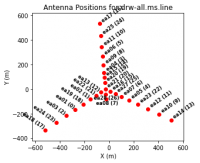
Next, we will look at a graphical plot of the antenna locations using the task plotants (see Figure 3a,b) and save an image copy to disk for later reference. This will be useful for selecting a reference antenna. Typically a good choice for a reference antenna is one close to the center of the array, but not too close to the center that it suffers from shadowing. The VLA "D" and "C" array configurations are particularly susceptible to shadowing at low elevations.
plotants(
    vis=vis_base,
    figfile="ant_locations_logspaced.png",
    logpos=True,
    antindex=True,  # shows numeric antenna index next to name, e.g. "ea08 (7)"
)
Based on its location alone, ea08 is a good candidate reference antenna because it is near the center of the array but it is unlikely to be shadowed because it is the furthest south among the North Arm antennas. The inner-most antennas of the West and East arms, ea13 and ea16, respectively, are also good choices. Our choice of reference antenna is contingent on that antenna having good data quality, which is something we will find as we more thoroughly inspect the data. Thus it is good to have several candidate reference antennas that one may choose from in the event that the first choice is problematic.
Plotting elevation versus time
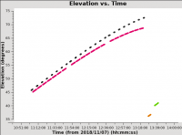
We will next look at the elevation as a function of time for all sources (see Figure 4) using the plotms tool (see the Data Examination/Editing page as well). Because we will frequently be sub-selecting the visibility data based on channel and polarization, we assign the selections to variables that we re-use throughout this tutorial.
The edge channels of sub-bands or spectral windows are often significantly noisier than the central channels, so we exclude the first three and last three channel, corresponding to channel indices 0, 1, 2, 61, 62, and 63 through the selection string "3~60" (ranges are end-inclusive). Since we exclude six channels, there are 58 channels out of 64 to include when averaging over the spectral window. We also assign a variable for when selecting the parallel hand polarizations (RR and LL) in order to exclude the cross-hand polarizations (RL and LR). We also assign a variable for a very long time interval for when effectively averaging over the whole dataset. Note that the edge channels, etc., are kept in this tutorial dataset for completeness and to act as examples for selecting data, but for one's own datasets one may wish to consider using split or mstransform to create a new MS that only includes the visibilities one wishes to calibrate.
spw0 = "0:3~60"
spw1 = "1:3~60"
all_spw = "0~1:3~60"

n_chan_in_range = "58"
n_chan_per_spw = "64"

parallel_hands = "RR,LL"
long_time = "1e8"  # seconds; ~3 years, effectively infinite
With those variables assigned, we now call plotms on our MS (assigned to the variable vis_base) to plot time on the x-axis versus elevation on the y-axis. Figure 4 shows the resulting plot, which also saved to the image file uncal_elevation_time.png. The gain calibrator (J0954+1743) is shown in black, IRC+10216 in magenta, bandpass calibrator (J1229+0203) in orange, and flux calibrator (3C286) in green. The observations span a bit under three hours in duration.
plotms(
    vis=vis_base,
    xaxis="time",
    yaxis="elevation",
    correlation=parallel_hands,
    spw=all_spw,
    coloraxis="field",
    # the parameters below are included to save the plot as a PNG file
    plotfile="uncal_elevation_time.png",
    highres=True,
    overwrite=True,
)
While it's not the case for these data, you may want to flag data when the elevation is very low (usually at the start or end of an observation). Also note that the proximity in elevation of the flux calibrator to the target will impact the ultimate absolute flux density calibration accuracy. Here, the flux and bandpass calibrators have been put at the end of the scheduling block in order to be as close to the target in elevation as is feasible given their LST ranges. This is somewhat sub-optimal because the absolute flux calibration will now be strongly dependent on the corrections for atmospheric opacity and the antenna elevation-gain curves. Thus this is something to keep in mind when planning observations. We will now turn to applying these calibration corrections.
Prior calibrations
Here we apply antenna calibration steps that use known information or existing model data. In the following steps we correct for known antenna position offsets, antenna elevation gain-curves, and atmospheric opacity. The calibration tables used to store the corrections are generated using the tasks gencal and plotweather. We then apply the calibration solutions to the data using the task applycal. Lastly, because we are unlikely to need to reverse these steps, we split out the corrected visibility data into a new measurement set that we use for further work in this tutorial.
Antenna Position Corrections
When antennas are moved in the array, their position may not be accurately known until a baseline solution has been determined at the telescope. In that case, the offset positions are published a few days after the observations and stored in a machine readable table accessible to CASA. This calibration step is done to determine if there are offsets and apply them if present. As mentioned in the observing log above, antenna 27 (ea27) was recently moved and has updated position data. We thus should check for any improved baseline positions derived after the observations were taken.
These corrections can be derived for the VLA using the CASA task gencal. The parameter caltype='antpos' will use antenna position offset values and create a calibration table ("cal.ant") for the delay changes that this correction involves. If the 'antenna' parameter is not specified, gencal will query the VLA webpages for the offsets (see the VLA Baseline Corrections page).
gencal(
    vis=vis_base,
    caltable="cal.ant",
    caltype="antpos",
    antenna="",
)
The above gencal call prints the antenna offsets to the logger:
Determine antenna position offests from the baseline correction database
offsets for antenna ea02 : -0.00060   0.00220  -0.00130
offsets for antenna ea04 :  0.00150   0.00190  -0.00150
offsets for antenna ea06 :  0.00120   0.00190  -0.00140
offsets for antenna ea13 :  0.00110   0.00120  -0.00140
offsets for antenna ea16 :  0.00110   0.00120  -0.00180
offsets for antenna ea20 : -0.00190   0.00110  -0.00130
offsets for antenna ea25 : -0.00340   0.00190  -0.00280
We can see that several antennas benefit from updated position data. The lack of an entry ea27 suggests that the updated position data was included in time for the observation.
Please note: If you are reducing VLA data taken before 2010 March 01, you will need to set caltype='antposvla' . Before this date the automated lookup will not work and you will have to specify the antenna positions explicitly.
Antenna elevation gain curves
Antennas are not absolutely rigid, and thus their effective collecting area and net surface accuracy vary with elevation as gravity deforms the surface. Gain curve calibration involves compensating for the effects of elevation on the amplitude of the received signals at each antenna. This calibration is especially important for the four highest frequency VLA bands (Ku, K, Ka, and Q) where the deformations represent a greater fraction of the observing wavelength. If one's complex gain calibrator is near the target source, and the flux density scale calibrator is also observed at a similar elevation, then most of the elevation-based gain will be calibrated during normal calibration.
Gain curves are generated into a separate calibration table using the task gencal with the caltype='gc' . Currently only gain curves for the VLA are implemented and this option should not be used with other telescopes.
gencal(
    vis=vis_base,
    caltable="cal.gc",
    caltype="gc",
)
Atmospheric opacity
Attenuation due to atmospheric opacity is significant for high frequency observations (>12 GHz) and is important to correct for proper flux density scaling. This is especially important if the flux calibrator and the targets are observed at different elevations. For lower frequencies (<12 GHz) this effect is marginal, and opacity correction is usually skipped.
The zenith opacity at the time of observation is computed for each subband from a combination of (a) weather station data and (b) a seasonal model. To account for the increased airmass at a particular elevation [math]\displaystyle{ el }[/math], the zenith opacity [math]\displaystyle{ \tau_z }[/math] are scaled using the expression [math]\displaystyle{ \exp[(-\csc[el]\tau_z)] }[/math]. This scaling is done automatically by the task gencal.
To start, we use the task plotweather to plot the atmospheric opacity as a function of frequency at the time of observation along with other diagnostic weather data. The plotweather task also returns the zenith opacities for each subband based on a weighted averaged of local weather station data and long-term statistics at the VLA site (the "weather model"; see Figure 5). The parameter seasonal_weight=0.5 gives both estimates equal weight.
Below we call the plotweather task and assign the list of opacities to the variable zenith_opacities, which will use further below. The opacity values are entered per spectral window in ascending frequency order.
zenith_opacities = plotweather(
    vis=vis_base,
    seasonal_weight=0.5,
    plotName="weather.png",
)
including the following opacity values printed to the logger:
SPW : Frequency (GHz) : Zenith opacity (nepers)
 0  :   36.312  :  0.041
 1  :   36.394  :  0.041
wrote weather figure: weather.png
The above call will also also create an image file weather.png in the current working directory showing the (1) elevation of the sun, (2) wind speed and direction, (3) air temperature, and (4) precipitable water vapor (PWV) as functions of time over the observation period. To view this file, use one's preferred image viewer like gthumb, xv, or Preview. One can also type just the variable name at the CASA prompt to show its values:
zenith_opacities
and it echoes the following output for the values set per spectral window:
Out[..]: [0.04061505896043428, 0.04085016638355082]
We can now create a calibration table for the opacities via gencal with the calmode='opac' parameter; we can either input the opacities directly or use the zenith_opacities variable:
gencal(
    vis=vis_base,
    caltable="cal.tau",
    caltype="opac",
    spw="0,1",
    parameter=zenith_opacities,
)
Please note: Note that one may get a "SEVERE" error warning printed to the logger when running plotweather related to an out of date leap second table. For the purposes of this tutorial, it is safe to ignore this warning. It can be resolved by updating the CASA data repository.
Applying calibrations
With the calibration tables generated for antenna position offsets ("cal.ant"), elevation gain curves ("cal.gc"), and atmospheric opacity ("cal.tau"), we now apply them to generate the "corrected" data column in the measurement set from the existing "data" column. We then split the corrected data out into a new measurement set for further calibration below. This mainly done to both simplify managing the calibration tables and to provide a useful "check point" to return to, since it is unlikely that one will need to revert the prior calibrations done above. We first apply the gains derived in the prior calibration tables to the visibilities in the base measurement set using the task applycal.
applycal(
    vis=vis_base,
    gaintable=["cal.ant", "cal.gc", "cal.tau"],
    flagbackup=False,
)
We set the option flagback=False to avoid creating a separate flag-versions file containing the pre-applycal version of the flags. In this case, it is unnecessary because the given calibration tables are unlikely to be missing solutions that will in-turn flag visibilities (as is sometimes the case with gain and bandpass calibration). We now use the task split to split the newly corrected data (stored in the "corrected" data column) out into a new measurement set via split:
split(
    vis=vis_base,
    outputvis=vis_prior,
    datacolumn="corrected",
)
Note that this step may be repeated to recreate the measurement set from this point (one may safely delete an MS with the rmtables task).
Data inspection and flagging
After having applied the prior calibrations, we now turn to inspecting the visibility data for our calibrators. Because the solutions derived from the calibrators will be applied to the target, it is essential that these solutions do not include corrupted data or interference. After we are satisfied with the data quality for our calibrators, we can later turn inspecting and flagging our target data.
Two forms of corruption are straightforward to identify from an amplitude versus time plot: interference that creates intermittent, spuriously large amplitudes, and various instrumental problems that result in low amplitudes. These narrow bandwidth spectral windows in Ka Band appear to be free of radio frequency interference (RFI), so the former does not appear in this dataset. Details on how to flag RFI may be found in the CASA guide VLA CASA Flagging. Thus our first task is to look for any spuriously low amplitudes in our calibrators.
Plotting amplitude versus time
Next, we will look at all the source amplitudes as a function of time using plotms:
plotms(
    vis=vis_prior,
    xaxis="time",
    yaxis="amp",
    correlation=parallel_hands,
    spw=all_spw,
    avgchannel=n_chan_in_range,
    coloraxis="field",
    # figure output parameters
    plotfile="uncal_amp_time.png",
    highres=True,
    overwrite=True,
)
The results are shown in Figure 6. The coloraxis="field" parameter colorizes the visibilities by target with the gain calibrator (J0954+1743) shown in black, IRC+10216 shown in magenta, the bandpass calibrator (J1229+0203) shown in orange, and the flux scale calibrator (3C286) shown in light green.
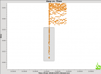
We can immediately see some low amplitude points at the start of the scans on J1229+0203 and 3C286, so we zoom in to inspect that data further. To zoom, select the Zoom tool ![]() in the lower left corner of the plotms GUI, then one can left click to draw a box. To unzoom, right click anywhere. A zoomed-in view of J1229+0203 is shown in Figure 7a. The low amplitude values appear on the first scan, so we use the Mark Region
in the lower left corner of the plotms GUI, then one can left click to draw a box. To unzoom, right click anywhere. A zoomed-in view of J1229+0203 is shown in Figure 7a. The low amplitude values appear on the first scan, so we use the Mark Region ![]() and Locate
and Locate ![]() buttons (positioned along the bottom of the GUI) to identify the source of the visibility points. The output will be shown in the logger. The first few entries of the selection are shown below:
buttons (positioned along the bottom of the GUI) to identify the source of the visibility points. The output will be shown in the logger. The first few entries of the selection are shown below:
Scan=56 Field=J1229+0203 [2] Time=2018/11/07/13:30:27.0000 BL=ea01@W06 & ea02@W04 [0&1] Spw=0 Chan=<3~60> Avg Freq=36.3155 Corr=LL X=5.04831e+09 Y=0.0221353 Observation=0
Scan=56 Field=J1229+0203 [2] Time=2018/11/07/13:30:27.0000 BL=ea02@W04 & ea07@E04 [1&6] Spw=0 Chan=<3~60> Avg Freq=36.3155 Corr=LL X=5.04831e+09 Y=0.0274988 Observation=0
Scan=56 Field=J1229+0203 [2] Time=2018/11/07/13:30:27.0000 BL=ea02@W04 & ea08@E01 [1&7] Spw=0 Chan=<3~60> Avg Freq=36.3155 Corr=LL X=5.04831e+09 Y=0.0292134 Observation=0
Scan=56 Field=J1229+0203 [2] Time=2018/11/07/13:30:27.0000 BL=ea02@W04 & ea14@E09 [1&13] Spw=0 Chan=<3~60> Avg Freq=36.3155 Corr=LL X=5.04831e+09 Y=0.0290748 Observation=0
Scan=56 Field=J1229+0203 [2] Time=2018/11/07/13:30:27.0000 BL=ea02@W04 & ea16@E02 [1&15] Spw=0 Chan=<3~60> Avg Freq=36.3155 Corr=LL X=5.04831e+09 Y=0.028712 Observation=0
Reviewing the complete set of entries shows a mix of antennas and correlation products (i.e., both RR and LL) but is otherwise limited to spectral window 0 and this first scan near 13:30:27 to 13:30:30 UT. We note this selection down for later flagging and now turn to inspecting the low-amplitude points seen in 3C286.
IMPORTANT NOTES ON PLOTMS:

* When using the locate button, it is important to have only selected a modest number
of points with the mark region tool (see example of marked region in the thumbnail),
otherwise the response will be very slow and possibly hang the tool
(all of the information will be output to your terminal window, not the logger).

* Throughout the tutorial, when you are done marking/locate, use the Clear Regions
tool to get rid of the marked box before plotting other things.

* After flagdata command flagging, you have to force a complete reload of the cache
to look at the same plot again with the new flags applied. To do this, either check
the "reload" box in the lower left before clicking Plot, or do Shift+Plot.

* Fields in the plotms GUI tabs can be altered and the data replotted
without having to close and restart plotms. After making changes, check the
Reload box and then click the Plot button adjacent to the Reload box.
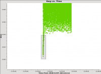
Click the "Clear Regions" ![]() button, and right click anywhere to go back to an un-zoomed view. Use the Zoom button to zoom-in on the lower values for 3C286 (green; Figure 7b). After locating the data points and reviewing the logger output, we again note no particular commonalities in antennas or correlation products, but that the data is otherwise limited to the spectral window 0 and the time range 13:38:54 to 13:39:00 UT.
button, and right click anywhere to go back to an un-zoomed view. Use the Zoom button to zoom-in on the lower values for 3C286 (green; Figure 7b). After locating the data points and reviewing the logger output, we again note no particular commonalities in antennas or correlation products, but that the data is otherwise limited to the spectral window 0 and the time range 13:38:54 to 13:39:00 UT.
Flagging low-amplitude time ranges
With the ranges of corrupted data identified above, we will now use flagdata to flag the data to exclude it from further analysis and calibration:
flagdata(
    vis=vis_prior,
    mode="list",
    inpfile=[f"field='{field_bandpass}' spw='0' timerange='13:30:27~13:30:30'",
             f"field='{field_flux}' spw='0' timerange='13:38:54~13:39:00'"],
)
Here we make use of the mode="list" parameter in flagdata to pass several flagging commands as separate strings in a Python list. The data selection will be connected by AND for each string. Because the time ranges are limited to a single a source, it is not necessary in principle to list the field entry, but when such commands are part of a script, this extra information can be useful to remind oneself which data one was flagging.
Plotting amplitude versus uv-distance
Next, look more closely at our science target, IRC+10216. We first plot visibility amplitude against time:
plotms(
    vis=vis_prior,
    xaxis="time",
    yaxis="amp",
    field=field_target,
    correlation=parallel_hands,
    avgchannel=n_chan_in_range,
    spw=all_spw,
    coloraxis="spw",
    # figure output parameters
    plotfile="uncal_amp_time_target.png",
    highres=True,
    overwrite=True,
)
Examining the output, we can see that there are some values with elevated noise, but no highly significant outliers. We next create a similar plot of amplitude against uv-distance:
plotms(
    vis=vis_prior,
    xaxis="uvdist",
    yaxis="amp",
    field=field_target,
    correlation=parallel_hands,
    avgchannel=n_chan_in_range,
    spw=all_spw,
    coloraxis="spw",
    # figure output parameters
    plotfile="uncal_amp_uvdist_target.png",
    highres=True,
    overwrite=True,
)
Because IRC+10216 has strong extended emission, we see higher amplitudes on the shortest uv-distance points. Again, we do not observe any significant outliers (see Figure 8). While this data has minimal (if any) RFI, it is generally advisable to wait until after calibration is complete to flag the target. The calibration procedures only require suitably well-flagged data for our calibrators and we then apply the calibration solutions to our target. When finished with the calibration, we will split out a new measurement set containing just the target visibilities. This creates a natural "check-point" for flagging, self-calibration, and continuum subtraction.
Set Up the Model for the Flux Calibrator
Next, we set the model for the flux calibrator. Depending on your observing frequency and angular resolution you can do this several ways. In the past, we typically used a point source (constant flux) model for the flux calibrator, possibly with a uvrange cut-off if necessary. More recently, model images for the most common flux calibrators have been made available for use in cases where the sources are somewhat resolved. This is most likely to be true at higher frequencies and at higher resolutions (more extended arrays).
The VLA flux calibrator models that are available in CASA can be checked through setjy:
setjy(
    vis=vis_prior,
    listmodels=True,
)
The terminal (not the logger) will now show the models, e.g., 3C286_C.im, 3C48_K.im, etc. Task setjy will search in the current working directory for images that may contain models, as well as in a CASA directory where known calibrator models are stored.
We will pick the Ka ('A') band model of 3C286: "3C286_A.im". Task setjy scales the total flux in the model image to that appropriate for your individual spectral window frequencies according to the calibrator's flux and reports this number to the logger. It is a good idea to save this information for your records. Note that due to a bug in CASA concerning the virtual model, we explicitly write to the model column in the MS below by setting the usescratch=True parameter.
setjy_results = setjy(
    vis=vis_prior,
    field=field_flux,
    scalebychan=True,
    model='3C286_A.im',
    usescratch=True,
)
The results are stored in the setjy_results Python dictionary and are also printed to the logger. The logger output for each spectral window is:
1331+305=3C286 (fld ind 3) spw 0  [I=1.7496, Q=0, U=0, V=0] Jy @ 3.6312e+10Hz, (Perley-Butler 2017)
1331+305=3C286 (fld ind 3) spw 1  [I=1.7466, Q=0, U=0, V=0] Jy @ 3.6394e+10Hz, (Perley-Butler 2017)
Using model image /home/casa/data/distro/nrao/VLA/CalModels/3C286_A.im
Scaling spw(s) [0, 1]'s model image by channel to  I = 1.74974, 1.7481, 1.74646 Jy @(3.63084e+10, 3.63537e+10, 3.63991e+10)Hz (LSRK) for visibility prediction (a few representative values are shown).
The absolute fluxes for the frequencies of all spectral window channels have now been determined, and we can proceed to the bandpass and complex gain calibrations.
Bandpass and Delay
Inspect the bandpass calibrator
Before determining the bandpass solution, we need to inspect phase and amplitude variations with time and frequency on the bandpass calibrator to decide how best to proceed. We limit the number of antennas to make the plot easier to see. We chose ea02 for the reference antenna as it seems like a good candidate. Let's try a single baseline to antenna ea23:
plotms(
    vis=vis_prior,
    field=field_bandpass,
    xaxis="channel",
    yaxis="phase",
    correlation=parallel_hands,
    avgtime=long_time,
    spw=spw0,
    antenna=f"{refant}&ea13",
)
The phase variation is modest ~10 degrees. Now expand to all baselines that include ea02, and add an extra dimension of color (see Figure 9):
plotms(
    vis=vis_prior,
    field=field_bandpass,
    xaxis="channel",
    yaxis="phase",
    antenna=refant,
    correlation=parallel_hands,
    avgtime=long_time,
    spw=spw0,
    coloraxis="antenna2",
    iteraxis="corr",
)
From this we can see that the phase variation across the bandpass for each baseline to antenna ea07 is modest. Next spw=1 for both correlations. Also check other antennas, if you like.
Now look at the phase as a function of time:
plotms(
    vis=vis_prior,
    field=field_bandpass,
    xaxis="time",
    yaxis="phase",
    correlation=parallel_hands,
    avgchannel=n_chan_in_range,
    spw=spw0,
    antenna=f"{refant}&ea13",
)
Expand to all antennas with ea02:
plotms(
    vis=vis_prior,
    field=field_bandpass,
    xaxis="time",
    yaxis="phase",
    antenna=refant,
    correlation=parallel_hands,
    avgchannel=n_chan_in_range,
    spw=spw,
    coloraxis="antenna2",
    iteraxis="corr",
)
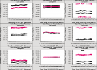
We can see the phase variations are smooth (see Figure 10), but do vary significantly over the 5 minutes of observation and in most cases by a few 10s of degrees (zoom in to see this better).
The conclusion from this investigation is that, especially for high frequency observations, we need to correct the phase variations with time before solving for the bandpass to prevent decorrelation of the vector averaged bandpass solution. Since the phase variation as a function of channel is modest (as noted in Figure 9), we can average over several (or all) channels to increase the signal to noise of the phase vs. time solution. If the phase variation, as a function of channel is larger, we may need to restrict averaging to only a few channels to prevent introducing delay-based closure errors as can happen from averaging over non-bandpass corrected channels with large phase variations.
Delay calibration
First, let's work on the delay calibration. The delay is the linear slope of phase across frequency. From the plot we saw that it was rather modest (the phases over frequency per baseline were aligned almost horizontal) and the bandpass calibration will certainly take care of it. Nevertheless, it is best to derive a delay calibration first and then calculate the bandpass. The delay calibration is an antenna based calibration solution and it can be derived in gaincal with parameter gaintype='K' .
gaincal_results = gaincal(
    vis=vis_prior,
    field=field_bandpass,
    caltable="cal.dly",
    refant=refant,
    refantmode="strict",
    gaintype="K",
)
We use the strong bandpass calibrator for the solution. It will be extrapolated in time to all observations.
Bandpass calibration
Now we proceed to the actual bandpass calibration. The first step is to correct for decorrelation. Since the bandpass calibrator is quite strong we do the phase-only solution on the integration time of 10 seconds (parameter solint='int' ).
gaincal_results = gaincal(
    vis=vis_prior,
    field=field_bandpass,
    refant=refant,
    refantmode="strict",
    caltable="cal.pbp",
    calmode="p",
    spw=all_spw,
    solint="int",
    gaintable=["cal.dly"],
)
This call also shows how the CASA calibration table system works. Calibration tables are incremental. By supplying the previous 'cal.dly' table as input to gaincal, we use it when calculating the present solutions. Note that the prior calibration tables were applied to the measurement and then split into a new dataset ("reduced_10s.ms.prior"); so the prior calibration tables (cal.ant, cal.gc, and cal.tau) need not be included.
Next we will plot the solutions with plotms (see Figure 11).
plotms(
    vis="cal.pbp",
    gridrows=3,
    gridcols=3,
    xaxis="time",
    yaxis="phase",
    iteraxis="antenna",
    plotrange=[0, 0, -180, 180],
    coloraxis="corr",
)
These solutions will appear in the CASA plotter GUI. If you closed it after plotting the antennas positions above, it should re-open. If it is still open from before, the new plots should just appear. After you are done looking at the first set of plots, push the Next button on the GUI to see the next set of antennas.
Now we can apply this phase solution on-the-fly while determining the bandpass solutions on the timescale of the bandpass calibrator scan (note parameter solint='inf' , which is the default).
bandpass(
    vis=vis_prior,
    field=field_bandpass,
    caltable="cal.bp",
    refant=refant,
    gaintable=["cal.dly", "cal.pbp"],
)
A few words about solint and combine:
The use of parameter solint='inf' in bandpass will derive one bandpass solution for the whole J1229+0203 scan. Note that if there had been two observations of the bandpass calibrator, this command would have combined the data from both scans to form one bandpass solution, because the default of the combine parameter for bandpass is combine='scan' . To solve for one bandpass for each bandpass calibrator scan we will use combine=' ' in the bandpass call. In all calibration tasks, regardless of solint, scan boundaries are only crossed when combine='scan' . Likewise, field and spw boundaries are only crossed if parameter combine='field' or parameter combine='spw' , respectively, are set. The latter two settings are not generally good ideas for bandpass solutions.
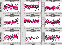
Plot the solutions, amplitude (see Figure 12) and phase (see Figure 13):
plotms(
    vis="cal.bp",
    gridrows=3,
    gridcols=3,
    xaxis="chan",
    yaxis="amp",
    iteraxis="antenna",
    coloraxis="corr",
)

plotms(
    vis="cal.bp",
    gridrows=3,
    gridcols=3,
    xaxis="chan",
    yaxis="phase",
    iteraxis="antenna",
    coloraxis="corr",
)
Note the scale for the phases, they are very small since the delays were already taken out in a previous calibration step (stored in cal.dly and used when it is included in gaintable).
Gain Calibration
Now that we have a bandpass solution to apply, we can solve for the antenna-based phase and amplitude gain calibration. Since the phase changes on a much shorter timescale than the amplitude, at least for the higher frequencies and/or longer baselines, we will solve for them separately. If the phase changes significantly over time and if the un-corrected phase were averaged over this timescale, the amplitude would decorrelate. Note that we now also re-solve for the gain solutions of the bandpass calibrator to derive new solutions that are corrected for the bandpass shape. Since the bandpass calibrator will not be used again, while not strictly necessary, it is useful to check its calibrated flux density.
gaincal_results = gaincal(
    vis=vis_prior,
    field=calibrator_fields,
    spw=all_spw,
    solint="int",
    caltable="cal.ign",
    calmode="p",
    refant=refant,
    refantmode="strict",
    gaintable=["cal.dly", "cal.bp"],
)
Here parameter solint='int' coupled with parameter calmode='p' will derive a single phase solution for each integration (recall, we averaged the data for every 10 seconds). Note that the bandpass table is applied on-the-fly before solving for the phase solutions, however the bandpass is NOT applied to the data permanently until applycal is run later on.
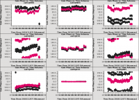
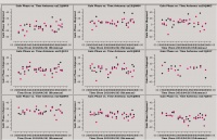
Now we will look at the phase solution, and note the scatter within a scan time (see Figure 14):
plotms(
    vis="cal.ign",
    gridrows=3,
    gridcols=3,
    xaxis="time",
    yaxis="phase",
    iteraxis="antenna",
    coloraxis="corr",
    plotrange=[0, 0, -180, 180],
)
Although solint='int' (i.e., the integration time of 10 seconds) is the best choice to apply before for solving for the amplitude solutions, it is not a good idea to use this to apply to the target. This is because the phase-scatter within a scan can dominate the interpolation between calibrator scans. Instead, we also solve for the phase on the scan time, solint='inf' (but combine=' ' , since we want one solution per scan) for application to the target later on. Unlike the bandpass task, the default of the combine parameter in the gaincal task is combine=' ' .
gaincal_results = gaincal(
    vis=vis_prior,
    field=calibrator_fields,
    spw=all_spw,
    solint="inf",
    caltable="cal.sgn",
    calmode="p",
    refant=refant,
    refantmode="strict",
    gaintable=["cal.dly", "cal.bp"],
)
And we then inspect the results (see Figure 15):
plotms(
    vis="cal.sgn",
    gridrows=3,
    gridcols=3,
    xaxis="time",
    yaxis="phase",
    iteraxis="antenna",
    coloraxis="corr",
    plotrange=[0, 0, -180, 180],
)
Alternatively, instead of making a separate phase solution for application to the target, we can also run smoothcal to smooth the solutions derived on the integration time.
Next we apply the bandpass and parameter solint='int' phase-only calibration solutions on-the-fly to derive amplitude solutions. Here the use of solint='inf' , not combine=' ' , will result in one solution per scan interval.
gaincal_results = gaincal(
    vis=vis_prior,
    field=calibrator_fields,
    spw=all_spw,
    solint="inf",
    caltable="cal.gn",
    calmode="ap",
    refant=refant,
    refantmode="strict",
    gaintable=["cal.dly", "cal.bp", "cal.ign"],
)
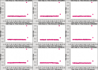
Now let's look at the resulting phase solutions (see Figure 16). Since we have taken out the phase as best we can by applying the solint='int' phase-only solution, this plot will give a good idea of the residual phase error. If we see scatter of more than a few degrees here, we should consider going back and looking for more data to flag, in particular for the times where these errors are large, or for other effects that may explain this behavior (and flag as necessary).
plotms(
    vis="cal.gn",
    gridrows=3,
    gridcols=3,
    xaxis="time",
    yaxis="phase",
    iteraxis="antenna",
    coloraxis="corr",
    plotrange=[0, 0, -10, 10],
)
Note that we have restricted the plot range so that all antennas are plotted with the same scale (instead of auto-scaled; for the X-axis the -1,-1 values still allow autoscaling; e.g., Figure 17). Here all of the antennas show reasonably small residual phases.
plotms(
    vis="cal.gn",
    gridrows=3,
    gridcols=3,
    xaxis="time",
    yaxis="amp",
    iteraxis="antenna",
    coloraxis="corr",
    plotrange=[-1, -1, 0, 1],
)
Note that because the bandpass and flux calibrators were observed at the end of the execution, their scans at the end show differing values. Antenna ea17 shows a slight dip in amplitude midway through the run, but is comparatively minor and well-tracked by the self-calibration.
Next we use the flux calibrator (whose flux density was set in setjy above) to derive the flux of the other calibrators. The flux table can be written as an incremental table, just like all other calibration tables. In that case it won't replace the cal.gn but both tables, cal.gn as well as cal.flx need to be carried onward.
fluxscale_results = fluxscale(
    vis=vis_prior,
    caltable="cal.gn",
    fluxtable="cal.flx",
    reference=field_flux,
    incremental=True,
)
It is a good idea to note the derived flux densities stored in the Python dictionary fluxscale_results, defined above, as well as printed to the logger:
Found reference field(s): 1331+305=3C286
Found transfer field(s):  J0954+1743 J1229+0203

Flux density for J0954+1743 in SpW=0 (freq=3.63155e+10 Hz) is: 0.292349 +/- 0.00501573 (SNR = 58.2865, N = 52)
Flux density for J0954+1743 in SpW=1 (freq=3.63982e+10 Hz) is: 0.294416 +/- 0.0050899 (SNR = 57.8432, N = 52)
Flux density for J1229+0203 in SpW=0 (freq=3.63155e+10 Hz) is: 15.2315 +/- 0.0152763 (SNR = 997.065, N = 52)
Flux density for J1229+0203 in SpW=1 (freq=3.63982e+10 Hz) is: 15.1615 +/- 0.0151884 (SNR = 998.224, N = 52)
Applycal and Inspect
Now we apply the calibration to each source with the derived tables and the appropriate source for that particular calibration. For the calibrators, all bandpass solutions are the same as for the bandpass calibrator (J1229+0203), and the phase and amplitude calibration as derived from their own visibility data.
Note: In all applycal steps we set calwt=False. It is very important to turn off this parameter which determines if the weights are calibrated along with the data. Data from antennas with better receiver performance and/or longer integration times should have higher weights, and it can be advantageous to factor this information into the calibration. Since these data weights are used at the imaging stage you can get strange results from having calwt=True when the input weights are themselves not meaningful, especially for self-calibration on resolved sources (e.g., flux density calibrator and target). For more recent data, the switched power information is recorded, but we currently do not recommend using this information to calculate data weights without exercising caution.
Next we apply the antenna position, antenna gaincurve, and opacity calibration, which are independent on source. We further apply the delay and bandpass as derived for source "5" (the other sources have no solutions for this in the table), and the short-term phase, amplitude and flux scaling that was determined from each calibrator source itself.
# Apply to the gain calibrator
applycal(
    vis=vis_prior,
    field=field_gain,
    gaintable=["cal.dly", "cal.bp", "cal.ign", "cal.gn", "cal.flx"],
    gainfield=2*[field_bandpass] + 3*[field_gain],
    calwt=False,
)
# Apply to the bandpass calibrator
applycal(
    vis=vis_prior,
    field=field_bandpass,
    gaintable=["cal.dly", "cal.bp", "cal.ign", "cal.gn", "cal.flx"],
    gainfield=5*[field_bandpass],
    calwt=False,
)
# Apply to the flux calibrator
applycal(
    vis=vis_prior,
    field=field_flux,
    gaintable=["cal.dly", "cal.bp", "cal.ign", "cal.gn", "cal.flx"],
    gainfield=2*[field_bandpass] + 3*[field_flux],
    calwt=False,
)
For the target we apply the bandpass, and the calibration from the gain calibrator using the scan length interval (cal.sgn):
applycal(
    vis=vis_prior,
    field=field_target,
    gaintable=["cal.dly", "cal.bp", "cal.sgn", "cal.gn", "cal.flx"],
    gainfield=2*[field_bandpass] + 3*[field_gain],
    calwt=False,
)
Now inspect the corrected data on the flux calibrator:
plotms(
    vis=vis_prior,
    xaxis="time",
    yaxis="amp",
    ydatacolumn="corrected",
    field=field_flux,
    avgchannel=n_chan_per_spw,
    iteraxis="antenna",
    correlation=parallel_hands,
)
and also on the gain calibrator:
plotms(
    vis=vis_prior,
    xaxis="time",
    yaxis="amp",
    ydatacolumn="corrected",
    field=field_gain,
    avgchannel=n_chan_per_spw,
    iteraxis="antenna",
    correlation=parallel_hands,
)
The corrected amplitudes are consistent in time and show no large deviations (see Figure 18 & 19). If we saw large deviations, we would select these using a rectangular region in plotms and inspect which antennas, spectral windows, and time ranges these visibilities come from using the Locate button. If there were large discrepancies here and in the proceeding plots, we would flag these data and repeat the steps from the bandpass calibration onward. New calls to applycal will overwrite the existing corrected data column, so the measurement set is fine to re-use as is for the re-application.
Now let's see how the target looks. Because the target has resolved structure, it's best to look at it as a function of uv-distance:
plotms(
    vis=vis_prior,
    xaxis="uvdist",
    yaxis="amp",
    ydatacolumn="corrected",
    field=field_target,
    avgchannel=n_chan_per_spw,
    coloraxis="antenna2",
    correlation=parallel_hands,
)
All values appear within a reasonable range. Note that because IRC+10216 is resolved, it shows higher flux values on shorter uv-distances, so this itself is not an issue.
Split
Now that calibration is complete, we split out the data for just the target. This is not strictly necessary, as we can select the appropriate fields when imaging, but is a good practice if we need to fall back and restart from this point. This can be useful if things go awry during continuum subtraction or self-calibration, for example. It also reduces the size of the measurement set in case we want to copy it to another machine or want to share the data with a colleague.
Here, we split off the target (IRC+10216). Note that to avoid a bug introduced in CASA 5.4.0 causing excessive flagging of the data (due to the combination of uvcontsub and statwt further on), we will exclude the cross-hand polarization products (RL and LR) in mstransform. As we will only make Stokes I maps of the sources, RL and LR are not used anyway in the below.
mstransform(
    vis=vis_prior,
    outputvis=vis_target,
    field=field_target,
    spw=all_spw,
    correlation=parallel_hands,
    keepflags=False,
)
This concludes the calibration phase of the data reductions.
UV Continuum Subtraction and Setting Up for Self-Calibration
In order to subtract the continuum to create a continuum-free data cube to image our spectral lines, we first need to identify the channels or frequencies associated with "off line" portions of the spectrum. We can make a first pass at this using a vector averaged plot of channel versus uv-amplitude using the calibrated data. It is important to note that we will only see signal in such a plot if (1) the data are well calibrated, and (2) there is significant signal near the phase center of the observations or if the line emission (or absorption) is weak but extended. If this isn't true for your data, you won't be able to see the line signal in such a plot and will need to make an initial (dirty or lightly cleaned) line+continuum cube to determine the line-free channels. Generally, this is the recommended course for finding the line-free channels more precisely than is being done here, as weak line signal would not be obvious in this plot.
plotms(
    vis=vis_target,
    xaxis="channel",
    yaxis="amp",
    correlation=parallel_hands,
    avgtime=long_time,
    avgscan=True,
    coloraxis="spw",
)
In the Display tab, change the Unflagged Points Symbol to Custom and Style to circle or diamond and 3 pixels.
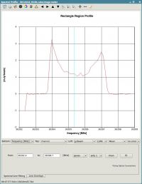
The horned profile typical of an expanding shell should be seen, as in Figure 21. From this plot, we can guess that strong line emission is restricted to channels 13 to 46 (zoom in if necessary to see exactly what the channel numbers are).
In the Data tab, under Averaging, we can also click on All Baselines to average all baselines, but this is a little harder to see.
Our aim is to use the line-free channels to create a model of the continuum emission that can be subtracted to create a line-only data set. We want to refrain from going too close to the edges of the band. These channels are typically noisy, and we don't want to get too close to the line channels because we could only see strong line emission in the vector averaged uv-plot and there may be weaker line emission in the channels next to the channel interval with strong lines.
We can now either specify the off line channels via the spectral window selection fitspec='0~1:3~13;46~60' and in uvcontsub via:
uvcontsub_results = uvcontsub(
    vis=vis_target,
    outputvis=vis_contsub,
    fitspec="0~1:3~13;46~60",
)
which excludes the line channels from the continuum fit. A new dataset will be written for irc10216.ms.contsub per the contents of the vis_contsub variable defined at the top of this tutorial. Note that this uses the new implementation of uvcontsub. The implementation available prior to CASA version 6.5.3 via the uvcontsub_old task.
Reweight the data
Before any imaging, it is good practice to remove the effects of relative noise scatter introduced by flagging uneven bits in the visibility data between the channels and times. Of course line emission affects this so the range of channels with line emission should be excluded in the noise determination. The task to weigh the data using noise statistics is statwt. Note that this split-off data set does not have a corrected data column anymore so we are using datacolumn = 'data' .
statwt_results = statwt(
    vis=vis_contsub,
    fitspw='0~1:14~45',
    excludechans=True,
    datacolumn='data',
)
The logger reports a mean value of 3.69 for the computed weights and a variance of 1.55.
Velocity Systems and Doppler corrections
Note that for spectral line observations where the Doppler shift of the line is greater than the width of a channel, we recommend using the cvel2 task. This step will correct for the Doppler shift during the observation. For this particular tutorial, the Doppler shift of the line is not wider than a channel, therefore we may skip this step.
The VLA WIDAR correlator does not support Doppler tracking, rather, Doppler setting is possible which will use the calculated sky frequency based on the velocity of a source at the start of the observation. The sky frequency is then fixed throughout that observing run. Typically, a fixed frequency is better for the calibration of interferometric data. The downside, however, is that a spectral line may shift over one or more channels during an observation. Task tclean, takes care of such a shift when re-gridding the visibilities in velocity space (default is LSRK) to form an image. Sometimes, in particular when adding together different observing runs, it may be advisable to re-grid all data sets to the same velocity grid, combine all data to a single file, then Fourier transform and deconvolve. The tasks cvel2, concat, and tclean serve this purpose respectively. The following run of cvel2 shows an example on how the parameters of cvel2 may be set.
To check the frequency span of the visibilities in the measurement set, we may refer to the listobs output generated near the beginning of this tutorial, or quickly check using the vishead task:
vishead(
    vis=vis_contsub,
    mode="summary",
)
which prints the following to the logger:
SpwID  Name           #Chans   Frame   Ch0(MHz)  ChanWid(kHz)  TotBW(kHz) CtrFreq(MHz) BBC Num  Corrs
0      EVLA_KA#B0D0#2     64   TOPO   36311.920       125.000      7250.0  36315.4822       15  RR  LL
1      EVLA_KA#B0D0#3     64   TOPO   36394.617       125.000      7250.0  36398.1795       15  RR  LL
For spectral window 0, this corresponds to about 1 km/s channel width. If we want to image the HC3N spectral line with a rest frequency of 36.39232 GHz over a velocity range of −50km/s to 0km/s and a channel width of 5 km/s, we may decide to re-grid the visibilities in cvel2 as:
vis_cvel = f"{vis_contsub}.cvel"

cvel2(
    vis=vis_contsub,
    outputvis=vis_cvel,
    spw="1",
    mode="velocity",
    nchan=10,
    start="-50km/s",
    width="5km/s",
    restfreq="36.39232GHz",
    outframe="LSRK",
    veltype="optical",
)
This will create a new data set where the data is binned into the new grid. Since all data in measurement sets are stored in frequency space, an inspection with vishead now gives:
vishead(
    vis=vis_cvel,
    mode="summary",
)
SpwID  Name           #Chans   Frame   Ch0(MHz)  ChanWid(kHz)  TotBW(kHz) CtrFreq(MHz)  BBC Num  Corrs
0      EVLA_KA#B0D0#3     10   LSRK   36392.927       606.974      6070.6  36395.6588        15  RR  LL
After the cvel2 step, the data can then be combined with other observations via concat and imaged in tclean with parameter specmode='cubedata' to conserve that velocity system and grid. Note that cvel2 can also Hanning smooth the data, if needed (as an alternative to the stand-alone hanningsmooth task).
Image the Spectral Line Data
The step above was for information purposes, for the tutorial we now go back to the split off data of the target source IRC+10216. This is the measurement set irc10216.ms.contsub which for the purposes of this guide we have stored in the variable vis_contsub. Since imaging can generally be a computationally intensive and time consuming task, especially for images with high angular resolution (i.e., many pixels) and many channels, it is generally good practice to first explore a limited selection of channels and then expand the analysis when we have a good idea of how best to proceed. Thus our imaging strategy is to (1) first image a few channels containing emission to assess, (2) image a few off-line channels to estimate the image noise, (3) interactively CLEAN a few channels with emission that we can use a reference, (4) apply automated imaging techniques to a few channels and compare their quality to the manually cleaned version from step-4, and finally (5) apply the automated techniques to the full cube. While our dataset is small and is in practice straightforward to image completely interactively from the start, these steps are meant to be a guide for more realistic, larger line imaging tasks that would be prohibitive to image manually (e.g., long tracks, multiple configurations, many spectral windows, many targets, etc.).
If you are starting mid-way through the guide using a measurement set that has already been calibrated, then these variables need to be assigned for the following commands to work correctly:
field_target = "IRC+10216"
vis_contsub = "irc10216.ms.contsub"
Creating a dirty image
We start by imaging a couple channels where emission is expected to be present to get a sense of how bright and extended the emission is. For other datasets, we may be concerned with whether emission is detected at all, although from the plot of amplitude versus channel (Figure 21) we know that strong emission is present from the get-go. We pick channel indices 18 and 19 for spectral window index 1 (HC3N), as they are especially bright in the averaged uv-data.
For imaging we will use the CASA task tclean to deconvolve the data. We'll start by generating a dirty map, i.e., one before any deconvolution has been applied and thus will contain significant artifacts from the sidelobes and structure of the synthesized beam. But, by having an image on hand before we attempt to interactively CLEAN, we can better assess the imaging parameters such as the image pixel size (cell size), size of the image (imsize), how far out to extend the primary beam mask, and other important quantities.
Note that interrupting tclean by Ctrl+C or by closing the viewer window may corrupt your visibilities or your CASA session when setting the parameter savemodel='modelcolumn' in 'tclean', as this option requires writing to the model column of the measurement set.
If cvel2 task was used in a previous step, then set the parameter specmode='cubedata', otherwise leave specmode='cube' within the tclean task.
Below we create a dirty image by calling tclean with zero minor cycle iterations by setting niter=0 such that it halts immediately after the image is created. The VLA Imaging topical guide has more information on the settings of the individual parameters of tclean. We also set variables for the line rest frequencies as a convenience.
restfreq_hc3n = "36.392238GHz"
restfreq_sis  = "36.309627GHz"

imagename_dirty = f"{field_target}_HC3N_dirty"
rmtables(f"{imagename_dirty}.*")
tclean(
    vis=vis_contsub,
    spw="1",
    imagename=imagename_dirty,
    imsize=[300, 300],
    cell="0.4arcsec",
    specmode="cube",
    outframe="LSRK",
    start=18,
    nchan=2,
    restfreq=restfreq_hc3n,
    perchanweightdensity=True,
    pblimit=-0.001,
    weighting="briggs",
    robust=0.5,
    niter=0,
    interactive=False,
);
It will take a moment to grid the data, and then write out the resulting image products. While we will use the CASA viewer for the interactive CLEAN procedures below, we use the CARTA application for viewing the resulting image. The CASA viewer is in the process of being deprecated, and while it will be maintained for the near future, CARTA is an excellent tool that already provides a superset of the viewer's functionality.
Figures 22 and 23 show the image and point spread function (PSF), respectively, for channel index 19. This is channel index 1 in the resulting cube since we started from 18 by way of the start parameter. We can also see that the PSF looks reasonable with the first sidelobes at at the ~15% level and the image quality looks promising. An especially poor PSF may result from miscalculating the weights, but here they look reasonable. While the authors of this guide had good estimates to begin with for the parameters passed to tclean, this would be a good stage to evaluate any changes. For example, depending on how faint or extended the emission is, we may elect to image the data with natural weighting instead of Briggs robust.
Measuring the image noise
We next image a subset of channels that are expected to not contain any emission to estimate the per-channel noise from. From Figure 21, we select channel indices 5 through 9. It is useful to know the thermal image noise because several stopping criteria are based on per channel estimates, and for channels with highly extended emission, the noise estimate is likely to be biased high. We can thus set absolute brightness limits to avoid channels that are insufficiently CLEANed.
imagename_noise = f"{field_target}_HC3N_noise"
rmtables(f"{imagename_noise}.*")
tclean(
    vis=vis_contsub,
    spw="1",
    imagename=imagename_noise,
    imsize=[300, 300],
    cell="0.4arcsec",
    specmode="cube",
    outframe="LSRK",
    start=5,
    nchan=4,
    restfreq=restfreq_hc3n,
    perchanweightdensity=True,
    pblimit=-0.001,
    weighting="briggs",
    robust=0.5,
    niter=0,
    interactive=False,
);
Inspecting this cube in CARTA, we can see that there appears to be no emission present. We next use the task imstat to estimate the RMS noise. Note that the noise can also be estimated by creating a region in CARTA and then checking the "statistics" tab. With imstat, the quantities are printed to the logger, and also returned in a variable that we extract the RMS value from below and print it.
noise_stats = imstat(imagename=f"{imagename_noise}.image")

rms = noise_stats["rms"][0]
print(f"RMS: {1e3*rms:.6f} mJy")
This reports a noise value of 0.97 mJy/beam. Note that this value depends on our channel width, which is relevant if one chooses to perform channel averaging on-the-fly in tclean.
Interactive CLEAN
Next we image the cube interactively for a few channels. Choose channels with bright, extended emission, since these are likely to require the most attention. We will use these manually CLEANed images as a basis for comparison when evaluating images created using automated techniques. Since the automated techniques require tuning various parameters, these manual images will act as a "ground truth" of sorts. Below we call tclean with the interactive=True parameter to image interactively. We also use the RMS calculated above (now set in the user-defined variable rms) to set a threshold at two times the RMS level using the threshold parameter. Since we know from the dirty image that there is a significant extended emission present, we use the multiscale deconvolver with scale sizes of a delta function (0 pixels), one half-power beamwidth, and three half-power beamwidth. By default tclean will resume CLEAN from an existing image, if it exists. Errors in CASA can occur when deleting an image that is open in the viewer or open in another process, so we use the rmtables task to check whether tables are open in another process before removing them.
imagename_interactive = f"{field_target}_HC3N_interactive"
rmtables(f"{imagename_interactive}.*")
tclean(
    vis=vis_contsub,
    spw="1",
    imagename=imagename_interactive,
    imsize=[300, 300],
    cell="0.4arcsec",
    specmode="cube",
    outframe="LSRK",
    start=19,
    nchan=1,
    restfreq=restfreq_hc3n,
    perchanweightdensity=True,
    pblimit=-0.001,
    weighting="briggs",
    robust=0.5,
    deconvolver="multiscale",
    scales=[0,5,15],
    threshold=f"{2*rms:.6f}Jy",
    niter=100_000,
    interactive=True,
);
The viewer will open when it's ready to start an interactive CLEAN.
Important: In the green menu on top, all polarizations for the clean mask. Select either the polygon region tool ![]() or the circular region tool. The lines drawn by the region tool will be green, making it difficult to see on the default rainbow color scheme image. The color map can be changed under the Data Display Options: click on the wrench icon or in the top menu, select Data, then select Adjust Data Display. Single clicks can be used to adjust the region and small squares will show anchor points that can be dragged to new positions. For the polygon region tool, single clicks will add new segments with anchor points on the vertices (shown as small green squares). A double click will connect the first and last vertices to create a polygon. Double click within the polygon to add the region to the CLEAN mask, which will be shown in white. To use the circular region tool instead, click and drag the bounding box of the circle over the source and adjust the anchor points on the corners to cover the emission. If you happen to mis-click, set the radio button to "Erase" instead of "Add", and the region will be subtracted from the CLEAN mask.
or the circular region tool. The lines drawn by the region tool will be green, making it difficult to see on the default rainbow color scheme image. The color map can be changed under the Data Display Options: click on the wrench icon or in the top menu, select Data, then select Adjust Data Display. Single clicks can be used to adjust the region and small squares will show anchor points that can be dragged to new positions. For the polygon region tool, single clicks will add new segments with anchor points on the vertices (shown as small green squares). A double click will connect the first and last vertices to create a polygon. Double click within the polygon to add the region to the CLEAN mask, which will be shown in white. To use the circular region tool instead, click and drag the bounding box of the circle over the source and adjust the anchor points on the corners to cover the emission. If you happen to mis-click, set the radio button to "Erase" instead of "Add", and the region will be subtracted from the CLEAN mask.
Note: If an interactive clean is started, and a mask is not created, then tclean will stop immediately, because in interactive sessions only emission within a mask is deconvolved. This is the opposite of a call to tclean with interactive=False, where without a mask the entire field of view will be deconvolved in an unrestricted fashion.
To continue with tclean use one of the Next action buttons in the green area on the Viewer Display GUI: The red "X" ![]() will stop tclean where it is; the blue arrow
will stop tclean where it is; the blue arrow ![]() will stop the interactive part of tclean, but continue to clean non-interactively until reaching the stopping niter (iterations x cycles) or threshold, whichever comes first. The green arrow
will stop the interactive part of tclean, but continue to clean non-interactively until reaching the stopping niter (iterations x cycles) or threshold, whichever comes first. The green arrow ![]() will clean until it reaches the iterations parameter on the left side of the green area. When the interactive viewer comes back use the tape deck to recheck that the mask encompasses what you think is real emission. If your mouse has a middle button, then by default it controls the image stretch.
will clean until it reaches the iterations parameter on the left side of the green area. When the interactive viewer comes back use the tape deck to recheck that the mask encompasses what you think is real emission. If your mouse has a middle button, then by default it controls the image stretch.
For this example, the threshold has been set to two times the RMS via the threshold parameter to avoid CLEANing too deeply. With a careful CLEAN mask you can CLEAN too close to the thermal noise limit (the actual observed RMS noise limit and not the theoretical one calculated for the proposal, as flagging, weather, etc., can affect what you actually get). It is optimal to CLEAN each channel of a cube to a specific threshold rather than stopping simply by exhausting the niter parameter, which can leave each channel cleaned to different levels. There are many ways to determine a suitable threshold. One way is to make a dirty image (niter = 0), open the cube using the viewer, go to a line free channel, select the box region tool, make a box near the field center about the size of your source, and double click inside.
Continue cleaning by using the green Next Action arrow ![]() until the residual displayed in the viewer looks noise-like. To speed things up, you might change the max_cycleniter parameter in the viewer. This parameter can also be set in the task command. The residual image shown in Figure 23 was obtained after creating a circular region and two rounds of 100 iterations, extending the region a bit using the polygon region toola nd two rounds of 500 iterations, and then a final round of 5000 iterations. You will notice that in this particular case there are residuals that cannot be cleaned. These residuals are due to the extended, resolved out structure on size scales larger than the array is sensitive to, or the Largest Angular Scale (LAS), that the array is sensitive to can be calculated from the shortest baseline length, and/or potential residual phase and amplitude calibration errors. We will explore this below in the section on self-calibration. The resulting restored image is shown in Figure 24.
until the residual displayed in the viewer looks noise-like. To speed things up, you might change the max_cycleniter parameter in the viewer. This parameter can also be set in the task command. The residual image shown in Figure 23 was obtained after creating a circular region and two rounds of 100 iterations, extending the region a bit using the polygon region toola nd two rounds of 500 iterations, and then a final round of 5000 iterations. You will notice that in this particular case there are residuals that cannot be cleaned. These residuals are due to the extended, resolved out structure on size scales larger than the array is sensitive to, or the Largest Angular Scale (LAS), that the array is sensitive to can be calculated from the shortest baseline length, and/or potential residual phase and amplitude calibration errors. We will explore this below in the section on self-calibration. The resulting restored image is shown in Figure 24.
Repeat the process for the SiS line using the call below. Note that the emission for this line is in spectral window index 0 and is less extended than the HC3N. The latter has to do with the different excitation situations of the two different lines. The SiS is excited closer to the central star than the HC3N. You may also notice that cleaning this cube takes many more iterations than the HC3N cube, so you may want to increase the iterations in the viewer (at the left in the green area at the top) or just stop before it ends by itself. Remember to select All Polarizations.
Automated masking
One could apply the manual, interactive procedures shown above to all of the channels, but this is generally laborious and time-consuming, especially if one has more than one target and spectral window to CLEAN. Thus we use the above files, namely the restored image, the CLEAN mask, and the residual, to help tune parameters for the automated masking procedures. Extensive parameter explorations have not been explored by NRAO staff for EVLA datasets, and thus typically require some tuning to give optimal results.
The masking algorithm we use is referred to as "auto-multithresh" which sets the CLEAN mask based on a combination of peak signal-to-noise in the image and what the current peak sidelobe level is. The image regions generated by these thresholds are then grown to lower signal-to-noise to extend the mask to fainter emission adjacent to more confident detections. This procedure of iteratively growing the mask down to a lower brightness threshold on each cycle roughly mimics the way in which most users generate masks manually: first making bright regions and then expanding the mask as those already CLEANed. Further information on the auto-multithresh algorithm and on tuning the parameters for optimal results can be found in the Automasking Guide. Note that quite often, good results can be achieved without any CLEAN mask at all, so it is worth trying this at least once before applying the automasking procedures.
The auto-multithresh algorithm tends to require a good amount of tuning on VLA data, so it is recommended to explore parameter combinations on a small number of representative channels (here channel 19) for faster iteration. For compact VLA configurations observing extended emission, part-way between the ALMA 12m and 7m array values offer a good starting point. Typically sidelobethreshold values are required for VLA observations than ALMA 12m or 7m observations. Below we start with values suitable for jointly imaged ALMA 12m and 7m ALMA observations with a noisethreshold=4.0 and sidelobethreshold=1.0:
imagename_autom = f"{field_target}_HC3N_autom"
rmtables(f"{imagename_autom}.*")
tclean(
    vis=vis_contsub,
    spw="1",
    imagename=imagename_autom,
    imsize=[300, 300],
    cell="0.4arcsec",
    specmode="cube",
    outframe="LSRK",
    start=19,
    nchan=1,
    restfreq=restfreq_hc3n,
    threshold=f"{1*rms:.6f}Jy",
    perchanweightdensity=True,
    pblimit=-0.001,
    weighting="briggs",
    robust=0.5,
    niter=100_000,
    interactive=False,
    # deconvolver
    deconvolver="multiscale",
    scales=[0, 5, 15],
    smallscalebias=0.5,
    # auto-multithresh
    usemask="auto-multithresh",
    noisethreshold=4.0,
    sidelobethreshold=1.0,
    minbeamfrac=0.3,
    lownoisethreshold=1.25,
    negativethreshold=1000.0,
    fastnoise=False,
);
The results are shown in Figure 25, which shows a sensible mask and a favorable image quality compared to our manually generated run.
Automated full-cube imaging
Now that we are happy with our results, we image the full cube. This will be a computationally expensive process, but one that requires little supervision from us now. For larger datasets, it often works well to "touch up" any minor defects in the automated run, such as missing faint extended emission in particularly complex channels, by restarting tclean on the image with interactive=True. Below we run tclean the same as above, except excluding the first channel (index 0) by setting start=1 and then image all channels onward by setting nchan=-1. This avoids an issue where the first channel, due to the velocity gridding and interpolation, will contain less data than the other channels and have a very degraded beam, causing issues for imaging the rest of the channels. The run should take approximately 12 major cycles.
imagename_full = f"{field_target}_HC3N_full"
rmtables(f"{imagename_full}.*")
tclean(
    vis=vis_contsub,
    spw="1",
    imagename=imagename_full,
    imsize=[300, 300],
    cell="0.4arcsec",
    specmode="cube",
    outframe="LSRK",
    start=1,
    nchan=-1,
    restfreq=restfreq_hc3n,
    threshold=f"{1*rms:.6f}Jy",
    perchanweightdensity=True,
    pblimit=-0.001,
    weighting="briggs",
    robust=0.5,
    niter=100_000,
    interactive=False,
    # deconvolver
    deconvolver="multiscale",
    scales=[0, 5, 15],
    smallscalebias=0.5,
    # auto-multithresh
    usemask="auto-multithresh",
    noisethreshold=4.0,
    sidelobethreshold=1.0,
    minbeamfrac=0.3,
    lownoisethreshold=1.25,
    negativethreshold=1000.0,
    fastnoise=False,
);
We now check the results by viewing (a) line-free channels to see if the masking and deconvolution was too aggressive on "noise spikes" in the image, and (b) checking other channels with strong emission to see how the masks and residuals compared. It is good practice to check both the restored image and residual together along with the CLEAN mask, which can be done in CARTA by selecting "Append" from the "File" menu. In Figure 26 we show another channel (index 29) with complex emission and in Figure 27 we show a channel (index 10) without emission. Both show good quality results without false positives or poor masks.
Image the Continuum data
For completeness, we image the continuum for the source as well. Below, we set the parameter specmode="mfs" in tclean to create a multi-frequency synthesis image out of all the non-line channels. Since the continuum image is typically quick and straightforward to image at high-frequency and narrow-band, we perform only one interactive CLEAN and create the CLEAN mask manually as above. Since no threshold is set, you will need to stop cleaning when the residual looks noise-like using the red "X" Next Action button ![]() (it will be done when the viewer comes back the second time). The continuum for IRC10216 is comparatively weak but interesting, tracing the photosphere of the AGB star.
(it will be done when the viewer comes back the second time). The continuum for IRC10216 is comparatively weak but interesting, tracing the photosphere of the AGB star.
imagename_cont = f"{field_target}_HC3N_cont"
rmtables(tablenames=f"{imagename_cont}.*")
tclean(
    vis=vis_target,
    spw="0~1:3~13;46~60",
    imagename=imagename_cont,
    imsize=[300, 300],
    cell="0.4arcsec",
    specmode="mfs",
    restfreq=restfreq_hc3n,
    perchanweightdensity=True,
    pblimit=-0.001,
    deconvolver="hogbom",
    weighting="briggs",
    robust=0.5,
    niter=100_000,
    interactive=True,
);
Note that to image the continuum, we use the line-free channels of the data before continuum subtraction, the name of which (irc10216.ms) is stored in the user-defined variable vis_target. We also select the line-free channels using a selection with the spw parameter. Careful observation will show that actually at least two weak lines are detected in our ostensibly line-free channels, so for real scientific applications it would be worthwhile to be more attentive to the channel selection. The resulting restored image is shown in Figure 28.
Moment maps
Maps of integrated intensity ("Moment 0"), intensity-weighted velocity ("Moment 1"), and intensity-weighted velocity dispersion ("Moment 2") can be generated using the immoments task. The name "moment" derives from an analogy to statistical moments in mathematics. Moment maps are especially useful for diagnostic purposes because the collapse (potentially large) three dimensional data cubes into two dimensional images. Moment maps can also be generated in CARTA (link).
In the example below we calculate Moments 0, 1, and 2 in addition to the maximum value (moment ID number 8). To avoid including excess noise in our moment calculation, which is especially problematic for Moments 1 and 2, we threshold the values to only include those above four times the image RMS, as specified by the includepix parameter below (1e8 is included as stand-in for infinity). Note that thresholding the Moment 0 map can bias it to higher flux values by way of including positive noise spikes and excluding the negatives. For presentation purposes, however, we apply the same thresholds to the Moment 0 map.
Below we call the immoments task that thresholds all values below four times the image RMS and creates the moments map simultaneously by supplying a list of moment map indices (detailed in documentation). We further sub-select the channels without significant emission to avoid adding undue noise to the statistical quantities. This can be determined by visually inspecting the cube.
immoments(
    imagename=f"{imagename_full}.image",
    chans="12~45",
    moments=[0,1,2,8],
    includepix=[4*rms, 1e8],
    outfile=imagename_full,
)
Note that the warnings about the kernel sampling may be safely ignored. The outfile parameter i used as the root name for the various images that are written out with file name extensions *.integrated, *.coordinate, *.weighted-coordinate, and .maximum.
For fun, you can download the VLT V-band image at http://casa.nrao.edu/Data/EVLA/IRC10216/irc_fors1_dec_header.fits kindly provided by Izan Leão and overlay the moment images and 36 GHz continuum (see Figure 30). More information about the dust properties can be found in the article Leão et al. (2006). For using the moment maps as masks or creating masks from them please refer to the Masking Images for Analysis page.
Position velocity diagrams
Position-velocity or "PV" diagrams are diagnostic plots that show the intensity of the emission as a function of position along a "cut" across the image plane (e.g., RA & Dec) and then project the frequency plane (e.g., velocity) into a new image. They are another useful tool for extracting a 2D view from a 3D data cube, which may be difficult to interpret on its own. They are also particularly useful because certain physical systems, such as a disk with Keplerian rotation or a spherically expanding shell, will show unique signatures in a PV diagram. In this section we show how to use the CASA task impv to create a PV diagram. One can also use CARTA (link) to generate PV diagrams interactively.
We first identify the position-slice to use to create the PV diagram from. In this example, for simplicity we open up the restored image in CARTA and create a line-type region and note the start and end image pixel coordinates. Instead of a list of numeric pixel values (e.g., [59, 162]), one may also specify the start and end positions as strings containing the WCS coordinates (e.g., ["9:47:59.87", "13:16:45.4"]). Figure 31 shows channel 19 from our restored image and the line region we've drawn in CARTA on top of it, which corresponds to the start x-y pixel [59, 162] and an end pixel [242, 162]. Note that to create a PV diagram in CARTA, one only needs to click the "PV" button from the list of icons at the top. To generate the PV diagram programmatically in CASA, we call impv to create the PV diagram as a new image:
imagename_pv = f"{field_target}_pv"
rmtables(f"{imagename_pv}.*")
impv(
    imagename=f"{imagename_full}.image",
    outfile=f"{imagename_pv}.image",
    start=[59, 162],
    end=[242, 162],
)
The resulting image is shown in Figure 32. The HC3N emission observed towards IRC+10216 originates from an (approximately) spherically expanding shell of ejecta. Such motions result in a circular pattern in a PV diagram, which we observe with textbook quality!
Spectrum Fitting
In addition to moment maps and PV-diagrams, model fitting functions, such as a Gaussian, is another common analysis task. This can be done with CASA's specfit task; specfit can fit those functions to an average spectrum defined by some area, or, alternatively, for each pixel. We will fit an average spectrum.
Fitting an Average Spectrum
First, we want to inspect the spectrum. Load the image into the viewer (select the HC3N image cube) and mark a region with the mouse button that is assigned to the rectangular R region in the tool bar. It is probably best to do this at a channel that shows the entire extent of the source (see Figure 30). When done, double click in the center of the box to see information about the image cube in the terminal and then select spectral profile from the Tools menu. The average spectrum will be displayed in a separate panel (see Figure 31).
To fit this profile in specfit, we need a region file outlining the 2-D region that is averaged (the magenta box in the viewer screenshot, Figure 30). In the following, we use the new CASA region format (CASA 3.3 and higher) that is described at the CASA Region Format page. Following the guidelines on that page, we create a file named specfit.crtf that describes a box with its [[x1,y1],[x2,y2]] corners in J2000 RA DEC coordinates. Use any text editor (e.g., emacs, vi, etc.) to create the file specfit.crtf with the CRTF identifier line as well as the following box parameters:
We will fit two Gaussians to the two peaks of the spectrum (the scientific merit is debatable). A file with initial values for the fit can be provided via the parameter estimates (see specfit' for more information). Here we will let CASA determine the start values by itself:
# Pseudo-interactive CASA
myfit = specfit(imagename='IRC10216_HC3N.cube.image',region='specfit.crtf',estimates='',ngauss=2)
Note that for the latter (pseudo-interactive CASA), the output is stored in a Python dictionary called "myfit", as well as printed to the CASA logger. You should get something similar to the following output, the results will vary based on your cleaning regions, depths, etc.:
Results for component 0:
    Type     : GAUSSIAN
    Peak     : 4.59 +/- 0.38 mJy/beam
    Center   : -16.60 +/- 0.41 km/s
               15.85 +/- 0.40 pixel
    FWHM     : 9.04 +/- 0.99 km/s
               8.77 +/- 0.96 pixel
    Integral : 44.2 +/- 6.1 mJy/beam.km/s
Results for component 1:
    Type     : GAUSSIAN
    Peak     : 3.82 +/- 0.32 mJy/beam
    Center   : -33.98 +/- 0.59 km/s
               32.72 +/- 0.57 pixel
    FWHM     : 13.4 +/- 1.5 km/s
               13.1 +/- 1.5 pixel
    Integral : 54.7 +/- 7.7 mJy/beam.km/s
We can see this seems to have caught the two peaks reasonably well.
Self-Calibration
The many different aspects of self-calibration could fill several CASA guides. Here we describe a simple process for this particular relatively low S/N data (low S/N per channel, at least).
While running tclean above, the model column for each channel will have been filled with the clean model (if you made a Fourier transform of this model, you would see an image of the clean components).
We choose to do the self cal on the spw=1 SiS line data because it has the strongest emission in a single channel and is a bit more compact than the HC3N data. We will run gaincal specifying the channel in the uv-data that has the brightest peak in the image (use the viewer to figure out which channel this is for spw=1), and note the peak flux. Since we started the image with a channel range, we need to account for the fact that the image channel numbers do not map exactly to the uv-data channel numbers (they are off by seven, so that channel index 12 (or e.g., 39) in the image is channel index 19 (or 46) in the uv-data).
Next we need to understand the S/N of the data. In particular, to self-cal, we need enough signal on a single baseline within the chosen solution interval, solint, to get a S/N of at least 3. We calculated above an average rms noise of about 2 mJy/beam/channel for the entire time range (about 95 minutes of on-source time) and all antennas (16). We can use our knowledge of the radiometer equation (see VLA Sensitivity) where rms scales as 1/sqrt(time * #baselines), and the number of baselines= N(N-1)/2 and N=# of antennas. So the rms noise on one baseline, for one 10 second integration in this observation is given by:
[math]\displaystyle{ {\rm RMS(baseline)} = {\rm 2\ mJy\ beam^{-1}\ channel^{-1}} \sqrt{ \frac{95\times 60\ {\rm sec}}{10\ {\rm sec}}\times\frac{16\times 15}{2\times 1}}\ {\sim}\ 500\ {\rm mJy\ beam^{-1}\ channel^{-1}} }[/math]
The 95 minutes of on-source time can be estimated from a plot where we can sum up the amount of time on a source (see Figure 32):
# Pseudo-interactive CASA
plotms(vis='day2_TDEM0003_10s_norx',field='3',ydatacolumn='corrected',
       xaxis='time',yaxis='amp',correlation='RR,LL',
       avgchannel='64',spw='1:4~60',antenna='')
This analysis suggests that the rms noise on one baseline, for one 10 second integration, is about 500 mJy. In contrast, the peak flux density in the strongest SiS channel is only about 200 mJy (this can be checked using the viewer). Since the emission is fairly compact, most baselines will see approximately this peak flux. This is why we choose the more compact of the two possible lines. Thus, a 10 second solution interval is not enough to get a SNR of at least 3 on a 200 mJy peak. We need to use a solint large enough so that the rms noise is not worse than about 1/3 of 200 mJy. Thus, a solint of 10 minutes is about the shortest we can use and be reasonably confident of the solutions.
Now we run gaincal with the solint we have determined. Note that because our desired solint is more than the scan time, we need to include parameter combine='scan' .
# Pseudo-interactive CASA
gaincal(vis='IRC10216.contsub',caltable='pcal_ch19one_10min',
        spw='1:19',calmode='p',solint='10min',combine='scan',
        refant='ea02',minsnr=3.0)
Next, look at the solutions:
# Pseudo-interactive CASA
plotms(vis='pcal_ch19one_10min',gridrows=3,gridcols=3,
         xaxis='time',yaxis='phase',iteraxis='antenna',
         coloraxis='corr',plotrange=[0,0,-50,50])
For some antennas we can see some trends away from zero: ea08 and ea27 are examples, and we can also see some smaller variations with time (see Figure 33).
Now we explore whether applying this solution actually improves matters. To do this, run applycal to apply the solutions to the line data set for both spw. We will set the interpolation parameter to use linearPD, this scales the phases by the frequency offset for the different spw. We only set linearPD for spw=0, since we derived the solutions for spw=1 in the above gaincal task. Use parameter spwmap to tell it that the solutions derived for spw=1 should be applied to both spw=0 and spw=1. Again, it's important to set parameter calwt=False.
# Pseudo-interactive CASA
applycal(vis='IRC10216.contsub',field='',spw='0,1',interp=['linearPD',''],
        gaintable=['pcal_ch19one_10min'],spwmap=[[1,1]],calwt=False)
Note: In this example, we ran the self-cal steps on the full uv continuum subtracted spectral line data set. For a more complex iterative self-calibration procedure, you may find it easier to split off the channel/spw you want to experiment on with split, and then do all the imaging (tclean) and gaincal steps with it. The gaincal tables created on the single channel can still be applied with applycal to the multi-channel/spw data set. If you do this, keep in mind that once split, the single-channel data will have its spw ID reset to 0 (you can check with listobs), no matter what spw it came from. Thus, in order to applycal with it, you would need parameter spwmap=[[0,0]].
To save time, we will use the clean mask we made before and run in a non-interactive mode. We can use a mask over again as long as the number of channels in the tclean call haven't changed. We can change cell or imsize and it will still do the right thing.
# Pseudo-interactive CASA
tclean(vis='IRC10216.contsub',spw='0:7~58',imagename='IRC10216_HC3N.cube.pselfcal',
       imsize=300,cell=['0.4arcsec'],specmode='cube',outframe='LSRK',restfreq='36.39232GHz',
       weighting='briggs',pblimit=-0.0001,perchanweightdensity=True,robust=0,
       niter=100000,threshold='3.0mJy',mask='IRC10216_HC3N.cube.mask')
# Pseudo-interactive CASA
tclean(vis='IRC10216.contsub',spw='1:7~58',imagename='IRC10216_SiS.cube.pselfcal',
     imsize=300,cell=['0.4arcsec'],specmode='cube',outframe='LSRK',restfreq='36.30963GHz',
     weighting='briggs',pblimit=-0.0001,perchanweightdensity=True,robust=0,
     niter=100000,threshold='3.0mJy',mask='IRC10216_SiS.cube.mask')
Now investigate the original and self-calibrated images in the viewer. We will find that even this single self-cal step significantly improves the images. Try opening both versions of the SiS image cubes. Select a bright channel via the tape deck controls, then use the wrench and pwrench tools to make a plot setting the same image range for both cubes, and two panels in x, then to see both images of that channel side-by-side click the blink toggle.
Figure 34: Original and self-cal SiS images for channel index 13/52 (zoomed in once), notice the increase in peak flux.
Repeat for HC3N (see Figure 35):
Figure 35: Original and self-cal HC3N images for channel index 23/52 (zoomed in once).
Now we can redo the moment images with the improved cubes. Be sure to change the output file names.
If you want to use the self-calibration solutions of the line data on the continuum, use the following:
# Pseudo-interactive CASA
applycal(vis='IRC10216',field='',spw='0,1',gaintable=['pcal_ch19one_10min'],spwmap=[[1,1]],calwt=False)

tclean(vis='IRC10216',spw='0~1:4~14,0~1:51~60',imagename='IRC10216.36GHzcont.pselfcal',
       imsize=300,cell=['0.4arcsec'],specmode='mfs',weighting='briggs',niter=100000,
       pblimit=-0.0001,robust=0,threshold='0.5mJy',mask='IRC10216.36GHzcont.mask')
Note that using the self-calibration of the extended line does not necessarily make the continuum better; it may seem like the imperfection of using the extended line channel has imprinted on the continuum.
All Commands Summarized
These commands were used in this tutorial.
To obtain the data first run these lines in a shell or terminal:
wget http://casa.nrao.edu/Data/EVLA/IRC10216/TDRW0001_10s.tar.gz
tar -xzf TDRW0001_10s.tar.gz
casa -r 6.5.3.28
Now run the following commands in an interactive CASA session:
TODO
Questions about this tutorial? Please contact the NRAO Science Helpdesk.
Last checked on CASA Version 6.4.1

