VLA CASA Pipeline-CASA4.5.3: Difference between revisions
| Line 108: | Line 108: | ||
In the first step, the data is imported from the SDM (Science Data Model) archival format to the CASA MeasurementSet (MS). Basic information on the MS is being provided, such as SchedBlock ID, the number of scans and fields and the size of the MS. The MS is also being checked for the scan intents and a baseline summary of the initial flags is obtained. | In the first step, the data is imported from the SDM (Science Data Model) archival format to the CASA MeasurementSet (MS). Basic information on the MS is being provided, such as SchedBlock ID, the number of scans and fields and the size of the MS. The MS is also being checked for the scan intents and a baseline summary of the initial flags is obtained. | ||
[[Image:VLApipe-importdata.png| | [[Image:VLApipe-importdata.png|150px|thumb|right|Fig. XX1: The ''hifv_importdata'' task page.]] | ||
In our example (Fig. XX1), a warning is issued that the data does not contain a CALIBRATE_BANDPASS scan intent. In this case, the pipeline will revert back to the flux density calibrator for bandpass calibration. | In our example (Fig. XX1), a warning is issued that the data does not contain a CALIBRATE_BANDPASS scan intent. In this case, the pipeline will revert back to the flux density calibrator for bandpass calibration. | ||
| Line 121: | Line 121: | ||
This step will apply online flags. That includes antennas not on source (ANOS), scans with intents that are of no use for the pipeline such as pointing and focus scans, autorrelations, the first and last three edge channels of each spw, clipping absolute zero values, quacking (ie removing the initial integration per scan), and flagging of entire basebands if needed. The flags are reported as a fraction of the total data for the full dataset as well as broken up into the individual calibrator scans as well as the target data. A plot is provided that displays the online antenna flags as a function of time. | This step will apply online flags. That includes antennas not on source (ANOS), scans with intents that are of no use for the pipeline such as pointing and focus scans, autorrelations, the first and last three edge channels of each spw, clipping absolute zero values, quacking (ie removing the initial integration per scan), and flagging of entire basebands if needed. The flags are reported as a fraction of the total data for the full dataset as well as broken up into the individual calibrator scans as well as the target data. A plot is provided that displays the online antenna flags as a function of time. | ||
[[Image:VLApipe-flagdata-big.png| | [[Image:VLApipe-flagdata-big.png|150px|thumb|right|Fig. XX3: The ''hifv_flagdata'' task page.]] | ||
In our example (Fig. XXX3), the target source is flagged from a start of 3.12% of the data, adding 6.05% due to antenna not on source, other online flags 0.82%, edge channels 6.4%, clipping 0.09% of absolute zero values, and 1.40% baseband clipping. This amounts to a total of 8.71% of flagging for the scientific target. Other sources are also listed and the entire MS was flagged on a 8.84% level. | In our example (Fig. XXX3), the target source is flagged from a start of 3.12% of the data, adding 6.05% due to antenna not on source, other online flags 0.82%, edge channels 6.4%, clipping 0.09% of absolute zero values, and 1.40% baseband clipping. This amounts to a total of 8.71% of flagging for the scientific target. Other sources are also listed and the entire MS was flagged on a 8.84% level. | ||
| Line 129: | Line 129: | ||
Step number 4 comprises the setting of the calibrator spectral and spatial model to the standard VLA flux density calibrators. The task page lists the flux densities of the calibrator model for each spw. | Step number 4 comprises the setting of the calibrator spectral and spatial model to the standard VLA flux density calibrators. The task page lists the flux densities of the calibrator model for each spw. | ||
[[Image:VLApipe-setjy.png| | [[Image:VLApipe-setjy.png|150px|thumb|right|Fig. XX4: The ''hifv_setjy'' task page.]] | ||
In our case, ''hifv_setjy '' throws an error ()Fig. XXX4) as ????????? | In our case, ''hifv_setjy '' throws an error ()Fig. XXX4) as ????????? | ||
| Line 138: | Line 138: | ||
Next, the prior calibration tables are being derived. They include gain-elevation dependencies, atmospheric opacity corrections, antenna offset corrections, and requantizer gains. They are independent of the calibrator scans themselves. | Next, the prior calibration tables are being derived. They include gain-elevation dependencies, atmospheric opacity corrections, antenna offset corrections, and requantizer gains. They are independent of the calibrator scans themselves. | ||
[[Image:VLApipe-precal1.png| | [[Image:VLApipe-precal1.png|150px|thumb|right|Fig. XX5a: The ''hifv_priorcals'' task page.]] | ||
[[Image:VLApipe-precal2.png| | [[Image:VLApipe-precal2.png|150px|thumb|right|Fig. XX5b: The ''hifv_priorcals'' task page.]] | ||
In addition to the opacities themselves (calculated per spw; Fig. XX5), a plot is attached that provides more information on the weather conditions during the observation. The antenna positions are usually updated days after the move and the corrections for four antennas in our case are in the millimeter range. | In addition to the opacities themselves (calculated per spw; Fig. XX5), a plot is attached that provides more information on the weather conditions during the observation. The antenna positions are usually updated days after the move and the corrections for four antennas in our case are in the millimeter range. | ||
| Line 148: | Line 148: | ||
Now it is time to determine the delays, and the bandpass solution (gain and phase). | Now it is time to determine the delays, and the bandpass solution (gain and phase). | ||
[[Image:VLApipe-testbpdcal.png| | [[Image:VLApipe-testbpdcal.png|150px|thumb|right|Fig. XX6: The ''hifv_testBPdcals'' task page.]] | ||
The plot on the main page (Fig. XX6) shows the flux density calibrator with the bandpass solution applied. The subpages show the delay, gain amplitude, gain phase, bandpass amplitude, and bandpass phase solutions for each antenna. Note that the phases will be close to zero for the reference antenna. When delays are more than +/-10ns it will be worth examining the data more closely. Some additional flagging may be needed. The gain apmlitude and phase solutions are derived per integration and they are used to correct for decorrelation for the spectral bandpass solutions. The latter are then determined over a full solution interval, usually for all bandpass scans together. Bandpasses should be smooth although they can vary substantially for wide frequency bands. The BP phases should capture the residuals after the delays are determined. | The plot on the main page (Fig. XX6) shows the flux density calibrator with the bandpass solution applied. The subpages show the delay, gain amplitude, gain phase, bandpass amplitude, and bandpass phase solutions for each antenna. Note that the phases will be close to zero for the reference antenna. When delays are more than +/-10ns it will be worth examining the data more closely. Some additional flagging may be needed. The gain apmlitude and phase solutions are derived per integration and they are used to correct for decorrelation for the spectral bandpass solutions. The latter are then determined over a full solution interval, usually for all bandpass scans together. Bandpasses should be smooth although they can vary substantially for wide frequency bands. The BP phases should capture the residuals after the delays are determined. | ||
Revision as of 10:55, 18 May 2016
Introduction
• With the start of Jansky VLA Full Operations (January 2013), we started a new operational model: – Deliver flagged and calibrated visibility data – You will self-calibrate and image visibility data to meet science goals, using resources at home institution or NRAO computing resources • Automated pipeline should run correctly on all “standard” Stokes I science SBs; “standard” means: – 128 MHz spws, but may work on other set-ups as well • Some constraints on strength of calibrators needed – Contains correctly labeled and complete scan intents • Current versions available: – “scripted” pipeline is a collection of python scripts that use CASA tasks wherever possible, but also uses toolkit calls; readable and easy to modify – CASA integrated pipeline is compatible with ALMA pipeline infrastructure, improved diagnostics in weblog, used as real-time pipeline since Sep 2015
=
• Real-time pipeline: – Minimal human intervention • Pipeline is run automatically on every science SB as it completes (not just “continuum”) – Pipeline output undergoes quality assurance checks by NRAO staff upon request; reports generated are archived as pipeline products • At your home institution: – Instructions for installation and operation of the VLA CASA Calibration Pipeline are available at https://science.nrao.edu/facilities/vla/data-processing/pipeline • Uses CASA 4.3.1, similar to current real-time pipeline • CASA 4.5.2 currently being validated (you are helping with this!) • Scripted pipelines for CASA versions through 4.5.0 also available – Provides more flexibility in how to use the pipeline, options suitable for spectral line datasets, mixed correlator set-ups, multi-band observations, etc. – Working to incorporate these into the CASA integrated pipeline
Pipeline Requirements
“Standard” Stokes I science SB means: – 128 MHz spws, but may work on other set-ups as well • Can work for narrower BWs, depends on the strength of the calibrators • Heuristics currently make some assumptions about the strength of the calibrators, in particular, the delay calibrator – Contains correctly labeled and complete scan intents • And also that the observation has been set up correctly! • Will the pipeline work for you? – The pipeline successfully completes on ~95% of all science SBs observed on the VLA; whether the output can be used for science depends on the science goal, and whether the observation was correctly set up • Pipeline includes Hanning smoothing, RFI flagging, and weight calculations that may not be appropriate for spectral line projects (but can modify scripted pipeline) • No polarization calibration (yet) but can use pipeline output as starting data for pol. cal. • Will probably work well for data taken since May 2012, may work for earlier EVLA data, likely that extra flagging may be needed in these cases
=
Calibrator strength: – Conservative limit on strength of BP and complex gain calibrators can be derived from requirement for initial gain calibration to work at high end of Q-band – Heuristic for delay calibration currently requires the SNR=3 limit on initial gain calibration per integration
=
• Correct observation set-up – Independent of whether you want to run the pipeline! – Remember: simple observing set-ups are always easier to calibrate – Do not skimp on calibration to spend more time on your target – you may end up not being able to calibrate the target data at all • Spending 3 minutes pointing could buy you more sensitivity than doubling the time on your target • Scan intents – The pipeline relies entirely on correct scan intents to be defined in each SB – In order for the pipeline to run successfully on an SB it must contain, at minimum, scans with the following intents: • A flux density calibrator scan that observes one of the primary calibrators (3C48, 3C138, 3C147, or 3C286) – this will also be used as the delay and bandpass calibrator if no bandpass or delay calibrator is defined • Complex gain calibrator scans
Overview of the Pipeline procedures
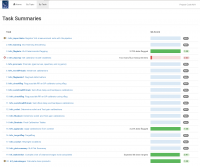
The pipeline is being executed in 20 individual pipeline tasks which are listed under the By Task tab (Fig. XXtasks). Each task has an associated score for success. But note that the scores are not implemented as of the CASA 4.5.3 VLA pipeline (C3R4B). Warnings and errors in tasks are also displayed by exclamation mark and cross icons next to the task names. In our example, the pipeline threw warnings in steps 1 and 20, and an error in step 4.
To obtain more details on each task execution, each tasks can be clicked on and the task results, including statistics, plots, and results can be examined. Common to each task page are details on the score (Pipeline QA; not implemented in the CASA VLA pipeline as packaged in 4.5.3), the task Input Parameters, Task Execution Statistics, and the associated CASA logs, which provide details on the actual commands that were issued as well as the associated logger outputs.
The pipeline steps are as follows:
1. hifv_importdata: Register VLA measurement sets with the pipeline
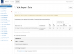
In the first step, the data is imported from the SDM (Science Data Model) archival format to the CASA MeasurementSet (MS). Basic information on the MS is being provided, such as SchedBlock ID, the number of scans and fields and the size of the MS. The MS is also being checked for the scan intents and a baseline summary of the initial flags is obtained.
In our example (Fig. XX1), a warning is issued that the data does not contain a CALIBRATE_BANDPASS scan intent. In this case, the pipeline will revert back to the flux density calibrator for bandpass calibration.
2. hifv_hanning: VLA Hanning Smoothing
This task runs Hanning-smoothes the MS. This is step will reduce the Gibbs phenomenon (ringing) when extremely bright and narrow spectral features are present, usually caused by strong rfi.
3. hifv_flagdata: VLA Deterministic flagging
This step will apply online flags. That includes antennas not on source (ANOS), scans with intents that are of no use for the pipeline such as pointing and focus scans, autorrelations, the first and last three edge channels of each spw, clipping absolute zero values, quacking (ie removing the initial integration per scan), and flagging of entire basebands if needed. The flags are reported as a fraction of the total data for the full dataset as well as broken up into the individual calibrator scans as well as the target data. A plot is provided that displays the online antenna flags as a function of time.
In our example (Fig. XXX3), the target source is flagged from a start of 3.12% of the data, adding 6.05% due to antenna not on source, other online flags 0.82%, edge channels 6.4%, clipping 0.09% of absolute zero values, and 1.40% baseband clipping. This amounts to a total of 8.71% of flagging for the scientific target. Other sources are also listed and the entire MS was flagged on a 8.84% level.
4. hifv_setjy: Set calibrator model visibilities
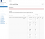
Step number 4 comprises the setting of the calibrator spectral and spatial model to the standard VLA flux density calibrators. The task page lists the flux densities of the calibrator model for each spw.
In our case, hifv_setjy throws an error ()Fig. XXX4) as ?????????
5. hifv_priorcals: Priorcals (gaincurves, opacities, and rq gains)
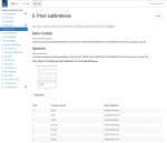
Next, the prior calibration tables are being derived. They include gain-elevation dependencies, atmospheric opacity corrections, antenna offset corrections, and requantizer gains. They are independent of the calibrator scans themselves.
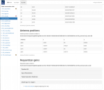
In addition to the opacities themselves (calculated per spw; Fig. XX5), a plot is attached that provides more information on the weather conditions during the observation. The antenna positions are usually updated days after the move and the corrections for four antennas in our case are in the millimeter range.
6. hifv_testBPdcals: Initial test calibrations
Now it is time to determine the delays, and the bandpass solution (gain and phase).
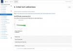
The plot on the main page (Fig. XX6) shows the flux density calibrator with the bandpass solution applied. The subpages show the delay, gain amplitude, gain phase, bandpass amplitude, and bandpass phase solutions for each antenna. Note that the phases will be close to zero for the reference antenna. When delays are more than +/-10ns it will be worth examining the data more closely. Some additional flagging may be needed. The gain apmlitude and phase solutions are derived per integration and they are used to correct for decorrelation for the spectral bandpass solutions. The latter are then determined over a full solution interval, usually for all bandpass scans together. Bandpasses should be smooth although they can vary substantially for wide frequency bands. The BP phases should capture the residuals after the delays are determined.
7. hifv_flagbaddef: Flag bad deformatters
8. hifv_checkflag: Flag possible RFI on BP calibrator using rflag
9. hifv_semiFinalBPdcals: Semi-final delay and bandpass calibrations
10. hifv_checkflag: Flag possible RFI on BP calibrator using rflag
11. hifv_semiFinalBPdcals: Semi-final delay and bandpass calibrations
12. hifv_solint: Determine solint and Test gain calibrations
13. hifv_fluxboot: Determine solint and Test gain calibrations
14. hifv_finalcals: Final Calibration Tables
15. hifv_applycals: Apply calibrations from context
16. hifv_targetflag: Targetflag
17. hifv_statwt: Reweight visibilities
18. hifv_plotsummary: VLA Plot Summary
19. hif_makeimlist: Compile a list of cleaned images to be calculated
20. hif_makeimages: Calculate clean products
Assuming requirements are met, the pipeline: – Loads the data – Hanning smooths** – Retrieves information about the observing set-up from the data – Applies deterministic flags (online flags, shadowed data, end channels of subbands, etc.) – Identifies primary calibrators and loads models – Derives all prior calibrations (antenna position corrections, gain curves, atmospheric opacity, requantizer gains) – Iteratively determines initial delay and bandpass solutions, including running RFLAG (RFI flagging algorithm), and identifying other system (deformatter) problems – Derives initial gain solutions, does flux density bootstrapping and derives spectral index of all calibrators
- May want to modify inputs and/or omit entirely for spectral line reductions
=
Heuristics (cont.): the pipeline: – Derives final delay, bandpass, and gain calibrations – Applies all calibrations to the MS – Runs RFLAG algorithm on all fields, including target** – Runs statwt to derive proper relative weights per antenna/spw**
- May want to modify inputs and/or omit entirely for spectral line reductions
• Pipeline products and output – Flag and calibration tables – Calibrated MS (available for 15 days, not archived) – Logs, including weblog used by quality assurance (QA) staff and QA report if requested
Data
Running the Pipeline
Assessing the Weblog
Pipeline Outputs
The real-time pipeline produces a calibrated and flagged MS for download (follow the directions in the email from the data analysts) – You may request a QA2 report from the data analysts – If you are happy with the pipeline calibration, then: • Do further flagging if necessary • Split out your target and image – If you have the SDM or uncalibrated MS and the calibration and flag tables, instructions for applying flags and calibration tables may be found at https://science.nrao.edu/facilities/vla/data-processing/pipeline • In some cases the pipeline and/or the MS may need to be modified – Download the SDM from the archive plus pipeline scripts – Follow the directions at above link • In some cases the pipeline heuristics may not be appropriate for your data (e.g., some L-band set-ups do not work well with the pipeline yet) – Reduce data by hand
Re-running the pipeline
Applying Pipeline Results
Known Issues and Workarounds
In general the pipeline does very well, but there are possible failure modes: – No flux density or gain calibrator intents defined, or flux density calibrator not one for which we have models • work around in scripted pipeline – Wrong scan intents • work around in scripted pipeline – Does not always identify deformatter problems (but does NOT usually have false positives – L-band may be an exception) • flag remaining bad spws – Calibrators are too weak for given spw bandwidth • heuristics have been developed and are currently being implemented
Incorrect scan intents
– Best to use the scripted pipeline (otherwise have to edit SDM)
– Can run through msinfo.py, then re-set the following string variables to
refer to the correct scan and field IDs:
flux_field_select_string='2'
bandpass_scan_select_string='8'
bandpass_field_select_string='4'
delay_scan_select_string='8'
delay_field_select_string='4'
calibrator_scan_select_string='4,5,7,8,10,11,12'
calibrator_field_select_string='1,2,3,4,5,6,7'
phase_scan_list=[1,3,5,7,9,11,13,15]
• If a standard flux density calibrator was not observed, you may still be able
to use the pipeline IF you know the flux density and spectral index of one
of your other calibrators, with a bit more work – contact the NRAO
helpdesk
Accurate flux density bootstrapping
– hifv_fluxboot uses medians to bootstrap flux densities: fairly robust, but in
some cases (e.g., high frequencies with pointing, elevation dependent gains) you
can do better by flagging the gain table used for the bootstrapping
– In scripted pipeline, run pipeline through fluxgains.py
– Flag gain table using “plotcal”
– Similar heuristic for the CASA pipeline currently being tested
– With care (match elevation of flux cal,
Spectral Line Data
Several steps in the real-time pipeline may not be appropriate for spectral line data: – Hanning smoothing (increases effective channel width) – Last run of RFLAG on target (may eliminate your line as interference!) – Statwt calculates rms based on scatter of channels per spw, per visibility; may want to run manually with channel selection turned on to eliminate use of channels containing line emission in calculating the rms • With the above modifications, the pipeline will work with spectral line data as long as the calibrators are strong enough
Polarization Calibration
Mixed Correlator Setups
With the new WIDAR capabilities it is common to observe both wide and narrow spws to obtain both continuum and spectral line data simultaneously, or multiple receiver bands – A single heuristic (e.g., gain calibration solution interval) for entire dataset may not be appropriate • Solution: – Run pipeline through application of deterministic flags, including Hanning smoothing if you are going to use it – Split the MS by spw and/or scans – Run pipeline on split MSs WITHOUT Hanning smoothing (you have already applied it, if you are going to use it) – Warning: output flagging statistics may not be correct
