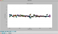
VLA CASA Bandpass Slope-CASA4.5.2
This CASA Guide is for CASA version 4.5.2
Overview
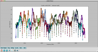
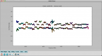
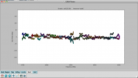
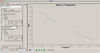
For the standard VLA flux calibrators, CASA includes a spatial and spectral model that is being applied for the and bandpass calibration. This model takes out the source characteristics and calibration solution then represent the instrument and atmospheric corrections. The VLA standards, however, have a relatively steep spectral index and are relatively weak at high frequencies. Although this is usually not a problem for absolute flux calibration, a good bandpass determination requires a very strong source, particularly for narrow channel widths. So for the high frequency, narrow channel case it is thus advisable to observe a different, but very strong source to correct for the bandpass. Such sources typically are variable and show a spectral slope that needs to be corrected for when the bandwidth is large. This tutorial describes how to model such a slope and correct the bandpass solution for it.
Data is taken in wide, 3-bit mode for the protostar G192.16-3.84 in Ka-band with spectral windows centered 29 and 36.5 GHz Each baseband has over 4 GHz of bandwidth comprised of 32 128-MHz spectral windows.
This is a more advanced tutorial, so if you are a relative novice, it is strongly recommended that you start with the EVLA Continuum Tutorial 3C391 (at least read it through), or even Getting Started in CASA before proceeding with this tutorial.
Obtaining the Data
As this tutorial concerns bandpass solutions only, we removed all other sources from the MS and only keep the bandpass calibrator scans. We also applied flagging and all pre-calibration steps including antenna position offsets, requantizer gains, opacity corrections, and gain-elevation curves. The original data (TVER0004.sb14459364.eb14492359.56295.26287841435) can be obtained through the [NRAO archive] and has a raw size of 57.04 GB.
The trimmed measurement set can be downloaded directly from http://casa.nrao.edu/Data/EVLA/G192/G192-BP.ms.tar.gz (dataset size: 2.1 GB)
Your first step will be to unzip and untar the file in a terminal (before you start CASA):
tar -xzvf G192-BP.ms.tar.gz
Starting CASA
As usual, to start CASA, type:
casa
This will run a script to initialize CASA, setting paths appropriately. It will also start writing to a file called ipython-<unique-stamp>.log, which will contain a record of all the text you enter at the CASA prompt, as well as casapy-<unique-stamp>.log, which will contain all the messages that are printed to the CASA logger window. It is recommended that you keep your log files in tact - you may need them to remind you of the last step you completed in your data reduction! (It is also a good idea to include your log files when submitting a help desk ticket).
Once CASA has started, a logger window will appear. Note that you can rescale this window or change the font size as desired (the latter is under "View").
Examining the Measurement Set (MS)
We use listobs to summarize our MS:
# In CASA: listobs on the initial data set
listobs('G192-BP.ms', listfile='G192_listobs.txt')
This will write the output to a file called G192_listobs.txt, which we can print to the terminal using the cat command:
# In CASA
cat G192_listobs.txt
We have trimmed to MS to contain only one scan on the bandpass calibrator 3C84, but retained all 64 spectral windows, each 128MHz wide and containing 128 1MHz channels.
Calibrating delays and initial bandpass solutions
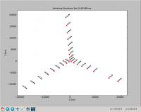
As a first step, we use an antenna that is near the center of the array and has a minimum of flags. The array can be mapped with plotants:
# In CASA: phase only calibration
plotants(vis='G192-BP.ms')
although the plot is a bit crowded, a zoom in shows that ea05 sits close to the center and appears to be a good choice.
First, we do a phase-only calibration solution on a narrow range of channels near the center of each spectral window on the bandpass calibrator 3C84 to flatten them with respect to time before solving for the bandpass. The range 60~68 should work. Pick a reference antenna near the center of the array -- ea05 is a reasonable choice (see above):
# In CASA: phase only calibration
gaincal(vis='G192-BP.ms', caltable='calG192.G0', \
        field='0', spw='*:60~68', \
        gaintype='G', refant='ea05', calmode='p', \
        solint='int', minsnr=3)
- refant='ea05' : Use ea05 as the reference antenna
- solint='int' : Do a per-integration solve (every 6 seconds, since we've time-averaged the data).
- minsnr=3 : Apply a minimum signal-to-noise cutoff. Solutions with less than this value will be flagged.
- gaintable is not set here as we have already applied pre-calibrations.
Plot the phase solutions (using full phase range, -180 to 180, instead of autorange):
# In CASA
plotcal(caltable='calG192.G0', xaxis='time', yaxis='phase', \
        iteration='antenna', plotrange=[-1,-1,-180,180])
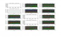
The first panel is blanked as ea01 is completely flagged. Step through the antenna-based solutions, here they look good (and fairly flat over the scans).
NOTE: When you are done plotting and want to use the calibration table in another task (e.g., for subsequent calibration or viewing with plotms), use the Quit button on the GUI to dismiss the plotter and free-up the lock on the calibration table. You should see a message in your terminal window saying "Resetting plotcal" which means you are good to go!
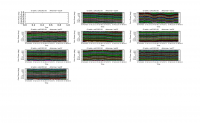
If you want to make single-page, multipanel plots (like those shown to the right), particularly for a hardcopy (where it only shows the first page), you can do:
# In CASA
plotcal(caltable='calG192.G0', xaxis='time', yaxis='phase', \
        antenna='0~10,12~15', subplot=531, iteration='antenna', \
        plotrange=[-1,-1,-180,180], fontsize=8.0, \
        markersize=3.0, figfile='plotG192_plotcal_G0p1.png')
plotcal(caltable='calG192.G0', xaxis='time', yaxis='phase', \
        antenna='16~26', subplot=531, iteration='antenna', \
        plotrange=[-1,-1,-180,180], fontsize=8.0, \
        markersize=3.0, figfile='plotG192_plotcal_G0p2.png')
We can now solve for the residual delays that we saw in plotms when we plotted phase vs. frequency. This uses the gaintype='K' option in gaincal. Note that this currently does not do a "global fringe-fitting" solution for delays, but instead does a baseline-based delay solution for all baselines to the reference antenna, treating these as antenna-based delays. In most cases with high-enough S/N to get baseline-based delay solutions, this will suffice. We avoid the edge channels of each spectral window by selecting channels 5~122:
# In CASA: residual delays
gaincal(vis='G192_flagged_6s.ms', caltable='calG192.K0', \
        gaintable=['calG192.antpos', 'calG192.gaincurve', 'calG192.requantizer', \
                   'calG192.opacity', 'calG192.G0'], \
        field='3', spw='*:5~122', gaintype='K', \
        refant='ea05', solint='inf', minsnr=3)
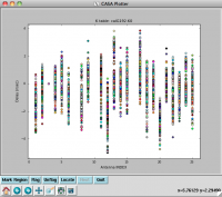
Note that we have also pre-applied our initial phase table, calG192.G0. We can plot the delays, in nanoseconds, as a function of antenna index (you will get one for each spw and polarization):
# In CASA
plotcal(caltable='calG192.K0', xaxis='antenna', yaxis='delay')
The delays range from around -5 to 4 nanoseconds.
Now we solve for the antenna bandpasses using the previous tables:
# In CASA: antenna bandpasses
bandpass(vis='G192_flagged_6s.ms', caltable='calG192.B0', \
         gaintable=['calG192.antpos', 'calG192.gaincurve', 'calG192.requantizer', \
                    'calG192.opacity', 'calG192.G0', 'calG192.K0'], \
         field='3', refant='ea05', solnorm=False, \
         bandtype='B', solint='inf')
WARNING: You must set solnorm=False here or later on you will find some offsets among spws due to the way the amplitude scaling adjusts weights internally during solving.
You will see in the terminal some reports of solutions failing due to "Insufficient unflagged antennas" -- note that these are for the channels we flagged earlier.
This is the first amplitude-scaling calibration that we do, so it is important to have used the calG192.gaincurve caltable (or set gaincurve=True) as well as the calG192.opacity caltable (or set opacity appropriately).
Plot the resulting bandpasses in amplitude and phase:
# In CASA
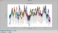
plotcal(caltable='calG192.B0', xaxis='freq', yaxis='amp', \
        spw='0~31', iteration='antenna')
#
plotcal(caltable='calG192.B0', xaxis='freq', yaxis='amp', \
        spw='32~63', iteration='antenna')
#
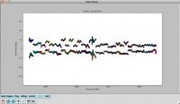
plotcal(caltable='calG192.B0', xaxis='freq', yaxis='phase', \
        iteration='antenna', spw='0~31', \
        plotrange=[-1,-1,-180,180])
#
plotcal(caltable='calG192.B0', xaxis='freq', yaxis='phase', \
        iteration='antenna', spw='32~63', \
        plotrange=[-1,-1,-180,180])
In the bandpass phases you no longer see the residual antenna delays (just residual spw phase offsets from the delay solution registration), but there are some band edge effects apparent.
Bootstrapping the bandpass calibrator spectrum
Unfortunately, our flux density calibrator was not bright enough at Ka-band to use as the bandpass calibration source. Since there is no a priori spectral information for our chosen bandpass calibrator, 3C84, we need to bootstrap to find its spectral index, then recalibrate with this information in order to avoid folding the intrinsic spectral shape of 3C84 into our calibration.
First, we use the initial round of bandpass calibration to create gain solutions for the flux and bandpass calibrators:
# In CASA: flux and bandpass calibrators gain
gaincal(vis='G192_flagged_6s.ms', caltable='calG192.G1', field='0,3', \
        gaintable=['calG192.antpos', 'calG192.gaincurve', 'calG192.requantizer', \
                   'calG192.opacity', 'calG192.K0', \
                   'calG192.B0'], \
        gaintype='G', refant='ea05', calmode='ap', solint='30s', minsnr=3)
Now let's have a look at the phase and amplitude solutions, iterating over antenna. We will look at the flux calibrator (3C147) and bandpass calibrator (3C84) individually since they're widely separated in time:
# In CASA
plotcal(caltable='calG192.G1', xaxis='time', yaxis='amp', \
        field='0', iteration='antenna')
#
plotcal(caltable='calG192.G1', xaxis='time', yaxis='amp', \
        field='3', iteration='antenna')
#
plotcal(caltable='calG192.G1', xaxis='time', yaxis='phase', \
        iteration='antenna', plotrange=[-1,-1,-180,180], \
        field='0')
#
plotcal(caltable='calG192.G1', xaxis='time', yaxis='phase', \
        iteration='antenna', plotrange=[-1,-1,-180,180], \
        field='3')
The solutions all look reasonable and relatively constant with time.
Now that we have gain solutions for the flux and bandpass calibrators, we can use fluxscale to scale the gain amplitudes of the bandpass calibrator:
# In CASA: bandpass calibrator gain amplitudes scaling
flux1 = fluxscale(vis='G192_flagged_6s.ms', caltable='calG192.G1', \
                  fluxtable='calG192.F1', reference='0', \
                  transfer='3', listfile='3C84.fluxinfo', fitorder=1)
- flux1 = fluxscale(...): by providing a variable flux1, we allow fluxscale to use this for the output Python dictionary it returns with lots of information about the flux scaling. You can inspect the output dictionary flux1 by typing "print flux1" at the CASA command line.
- fluxtable='calG192.F1': this is the output scaled gain table. Since we are only using this to find the spectral index of 3C84, we won't be using this table.
- listfile='3C84.fluxinfo': an output file that contains the derived flux values and fit information.
- fitorder=1: only find a spectral index, ignoring curvature in the spectrum.
The last line in the file (and displayed in the logger) shows:
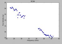
Fitted spectrum for 3c84-J0319+413 with fitorder=1: Flux density = 31.454 +/- 0.0310638 (freq=32.5128 GHz) spidx=-0.493668 +/- 0.00820698
Using the information in the returned flux dictionary, we can plot the derived spectrum:
# In CASA
freq = flux1['freq'] / 1e9
spw_list = range(0,64)
spw_str = []
for i in spw_list:
   thisspw = str(i)
   spw_str.append(thisspw)

bootstrapped_fluxes = []
for j in spw_str:
    thisflux = flux1['3'][j]['fluxd'][0]
    if thisflux ==None:
        continue
    else:
        bootstrapped_fluxes.append(thisflux)

pl.clf()
pl.plot(freq, bootstrapped_fluxes, 'bo')
pl.xlabel('Frequency (GHz)')
pl.ylabel('Flux Density (Jy)')
pl.title('3C84')
pl.show()
Note the bump around 37 GHz -- what is this? We will not be able to account for it with the simple spectral index model, but still, ours is a good first approximation.
We can use the model from fluxscale to fill the MODEL column with 3C84's spectral information using setjy:
# In CASA: spectral information
setjy(vis='G192_flagged_6s.ms', field='3', scalebychan=True, \
      standard = 'manual', fluxdensity=[29.8756, 0, 0, 0], spix=-0.598929, \
      reffreq='32.4488GHz')
Checking with plotms that the data have been appropriately filled:
# In CASA
plotms(vis='G192_flagged_6s.ms', field='3', antenna='ea05&ea02', \
       xaxis='freq', yaxis='amp', ydatacolumn='model')
Finally, we redo the previous calibration using this new model information. Although the commands are the same as what we issued earlier, keep in mind that the model values for the bandpass calibrator have changed, and therefore the results of these calibration calculations will differ:
# In CASA: phase only recalibration
gaincal(vis='G192_flagged_6s.ms', caltable='calG192.G0.b', \
        field='3', spw='*:60~68', \
        gaintable=['calG192.antpos', 'calG192.gaincurve', \
                   'calG192.requantizer', 'calG192.opacity'], \
        gaintype='G', refant='ea05', calmode='p', \
        solint='int', minsnr=3)
# In CASA: residual delays recalibration
gaincal(vis='G192_flagged_6s.ms', caltable='calG192.K0.b', \
        gaintable=['calG192.antpos', 'calG192.gaincurve', 'calG192.requantizer', \
                  'calG192.opacity', 'calG192.G0.b'], \
        field='3', spw='*:5~122', gaintype='K', \
        refant='ea05', solint='inf', minsnr=3)
# In CASA: antenna bandpasses recalibration
bandpass(vis='G192_flagged_6s.ms', caltable='calG192.B0.b', \
         gaintable=['calG192.antpos', 'calG192.gaincurve', 'calG192.requantizer', \
                    'calG192.opacity', 'calG192.G0.b', 'calG192.K0.b'], \
         field='3', refant='ea05', solnorm=False, \
         bandtype='B', solint='inf')
It's a good idea to inspect these solutions as well:
# In CASA
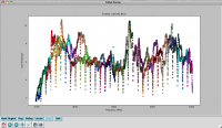
plotcal(caltable='calG192.B0.b', xaxis='freq', yaxis='amp', \
        spw='0~31', iteration='antenna')
#
plotcal(caltable='calG192.B0.b', xaxis='freq', yaxis='amp', \
        spw='32~63', iteration='antenna')
#
plotcal(caltable='calG192.B0.b', xaxis='freq', yaxis='phase', \
        iteration='antenna', spw='0~31', \
        plotrange=[-1,-1,-180,180])
#
plotcal(caltable='calG192.B0.b', xaxis='freq', yaxis='phase', \
        iteration='antenna', spw='32~63', \
        plotrange=[-1,-1,-180,180])
They look virtually unchanged from the previous solutions, with the exception that the amplitude scaling is corrected for the spectrum of 3C84. Now that we have the final version of our bandpass calibration, we can proceed to the full calibration of the dataset.
