TWHydraBand7 Imaging for CASA 3.3

Prepare Continuum Data for Further Processing

In order to speed up imaging/self-calibration for the continuum data we will average channels together, and then flag the few spectral features. This method works well in the case of only a few spectral lines, while retaining enough channelization to aid in multi-frequency synthesis and being able to remove spectral features in the averaged data. The amount of channel averaging should be adjusted to your particular data. Note for wide bandwidth data it is never a good idea to use the continuum estimate generated by uv-continuum subtraction as your continuum data. This worked OK in the past with the narrow band systems like the VLA and low dynamic range instruments like the SMA, but is not advised for ALMA wide bandwidth, high dynamic range data.

One can also flag the spectral features first but in that case make a backup of the file that is analogous to TWHydra_corrected.ms as you will need it later (unflagged) for spectral line imaging.

# In CASA
split(vis='TWHydra_corrected.ms',outputvis='TWHydra_cont.ms',
       spw='0~3:22~3820',width=100,datacolumn='data')

Now make a plot of amplitude vs. channel to see what needs to be flagged

# In CASA
plotms(vis='TWHydra_cont.ms',spw='0~3',xaxis='channel',yaxis='amp',
      avgtime='1e8',avgscan=T,coloraxis='spw',iteraxis='spw',xselfscale=T)

The CO(3-2) and HCO+(4-3) lines are obvious. The 4th spw; spw=3 also shows an upswing on the highest channels that is problematic, could be a weak atmospheric feature.

# In CASA
flagdata(vis='TWHydra_cont.ms',
         spw=['0:16~16','2:21~21','3:33~37'])

Have a look at the continuum as a function of uv-distance. If the data are flat as a function of uv-distance the source is completely unresolved. If you see structure (in this case decreasing amplitude with uv-distance) the source is resolved.

# In CASA
plotms(vis='TWHydra_cont.ms',spw='',xaxis='uvdist',yaxis='amp',field='',avgchannel='38',
       coloraxis='spw',iteraxis='spw')

Image and Self-Calibrate the Continuum

Make an initial image using clean. We use mode='mfs' to do multifrequency synthesis, in other words grid each uv-channel independently. Since the uv-spacing is a function of frequency, this will actually achieve greater uv-coverage than if all the channels and spws had been averaged in advance. The imsize=100 and cellsize=0.3arcsec were chosen to be appropriate for the Band and antenna configuration. At ALMA Band 7, the primary beam is about 30" and we want to image all of it. For the configuration used to take these data, the resolution is expected to be about 1.5" and it is a good idea to oversample the beam by a factor of 4 or 5 (we used 5 here).

For doing self-calibration it is essential that only "real" signal be included in the image model, thus it is important to make a clean mask, and clean the first iteration rather shallowly. In the example below we set interactive=T so you can interactively make the clean mask and stop clean when the signal from the source starts to approach the surrounding "noise" areas in the residual map.

# In CASA
clean(vis='TWHydra_cont.ms',imagename='TWHydra_contall',
      mode='mfs',calready=T,imagermode='csclean',
      imsize=100,cell=['0.3arcsec'],spw='',
      weighting='briggs',robust=0.5, 
      mask='',
      interactive=T,threshold='1mJy',niter=100000)

The parameter calready=T ensured that a uv-model of the resulting image was placed in the model data column. This model can then be used to self-calibrate the data using gaincal. We use gaintype='T' to tell it to average the polarizations before deriving solutions which gains us a sqrt(2) in sensitivity. A critical parameter to play with is solint, we use solint=30s to gain a bit of sensitivity. From listobs the integration time of these data are about 10 seconds, using solint=30s then gives us a sqrt(3) in sensitivity. It is often best to start with a larger solint and then work your way down to the integration time if the S/N of the permits. For the same reasons as described in the TWHydraBand7_Calibration tutorial we want to fix up the phases before tackling amplitude by setting calcode='p'.

# In CASA
gaincal(vis='TWHydra_cont.ms',caltable='self_1.pcal',
        solint='30s',combine='',gaintype='T',
        refant='DV06',spw='',minblperant=4,
        calmode='p',minsnr=2,)

# In CASA
applycal(vis='TWHydra_cont.ms',field='',
        gaintable=['self_1.pcal'],calwt=F)

# In CASA
clean(vis='TWHydra_cont.ms',imagename='TWHydra_contall_1pcal',
      mode='mfs',calready=T,imagermode='csclean',
      imsize=100,cell=['0.3arcsec'],spw='',
      weighting='briggs',robust=0.5, 
      mask='TWHydra_contall.mask',
      interactive=T,threshold='1mJy',niter=100000)

# In CASA
gaincal(vis='TWHydra_cont.ms',caltable='self_2.pcal',
        solint='30s',combine='',gaintype='T',
        refant='DV06',spw='',minblperant=4,
        calmode='p',minsnr=2,)

# In CASA
plotcal(caltable='self_2.pcal',xaxis='time',yaxis='phase',
        spw='',field='',antenna='1~8',
        iteration='antenna',subplot=421,plotrange=[0,0,-80,80])

# In CASA
applycal(vis='TWHydra_cont.ms',field='',
        gaintable=['self_2.pcal'],calwt=F)

# In CASA
clean(vis='TWHydra_cont.ms',imagename='TWHydra_contall_2pcal',
      mode='mfs',calready=T,imagermode='csclean',
      imsize=100,cell=['0.3arcsec'],spw='',
      weighting='briggs',robust=0.5, 
      mask='TWHydra_contall_1pcal.mask',
      interactive=T,threshold='1mJy',niter=100000)

# In CASA
gaincal(vis='TWHydra_cont.ms',caltable='self_ap.cal',
        solint='inf',combine='',gaintype='T',
        refant='DV06',spw='',minblperant=4,
        gaintable=['self_2.pcal'],
        calmode='ap',minsnr=2,)

# In CASA
plotcal(caltable='self_ap.cal',xaxis='time',yaxis='phase',
        spw='',field='',antenna='1~8',
        iteration='antenna',subplot=421,plotrange=[0,0,-1,1])

# In CASA
plotcal(caltable='self_ap.cal',xaxis='time',yaxis='amp',
        spw='',field='',antenna='1~8',
        iteration='antenna',subplot=421)

# In CASA
applycal(vis='TWHydra_cont.ms',field='',
        gaintable=['self_2.pcal','self_ap.cal'],calwt=F)

# In CASA
plotms(vis='TWHydra_cont.ms',xaxis='uvdist',yaxis='amp',
       avgchannel='38',ydatacolumn='corrected',iteraxis='spw')

# In CASA
plotms(vis='TWHydra_cont.ms',xaxis='time',yaxis='amp',iteraxis='spw',
       ydatacolumn='corrected')

# In CASA
clean(vis='TWHydra_cont.ms',imagename='TWHydra_contall_apcal',
      mode='mfs',calready=T,imagermode='csclean',
      imsize=100,cell=['0.3arcsec'],spw='',
      weighting='briggs',robust=0.5, 
      mask='TWHydra_contall_2pcal.mask',
      interactive=T,threshold='1mJy',niter=100000)

Continuum Subtraction and Spectral Line Imaging

Make channel plot to get line-free channel ranges. Since the line emission is simple in this case and there are more than enough line-free channels we do not need to be very precise just stay well away from the line and best to chose ranges on either side.

# In CASA
split(vis='TWHydra_corrected.ms',outputvis='TWHydra_CO3_2.ms',
      datacolumn='corrected',spw='2')

# In CASA
uvcontsub2(vis='TWHydra_CO3_2.ms',fitorder=1,fitspw='0:20~2000,0:2400~3800')

# In CASA
clean(vis='TWHydra_CO3_2.ms.contsub',imagename='TWHydra_CO3_2line',
      imagermode='csclean',calready=T,spw='',
      imsize=100,cell=['0.3arcsec'],
      mode='velocity',start='-4km/s',width='0.12km/s',nchan=118,
      restfreq='345.79599GHz',outframe='LSRK',
      weighting='briggs',robust=0.5,
      mask='',
      interactive=T,threshold='1mJy',niter=100000)

# In CASA
split(vis='TWHydra_corrected.ms',outputvis='TWHydra_HCOplus.ms',
      datacolumn='corrected',spw='0')

# In CASA
uvcontsub2(vis='TWHydra_HCOplus.ms',fitorder=1,fitspw='0:20~1500,0:1900~3800')

# In CASA
clean(vis='TWHydra_HCOplus.ms.contsub',imagename='TWHydra_HCOplusline',
      imagermode='csclean',calready=T,spw='',
      imsize=100,cell=['0.3arcsec'],
      mode='velocity',start='-4km/s',nchan=118,width='0.12km/s',
      restfreq='356.7342GHz',outframe='LSRK',
      weighting='briggs',robust=0.5,
      mask='',
      interactive=T,threshold='1mJy',niter=100000)

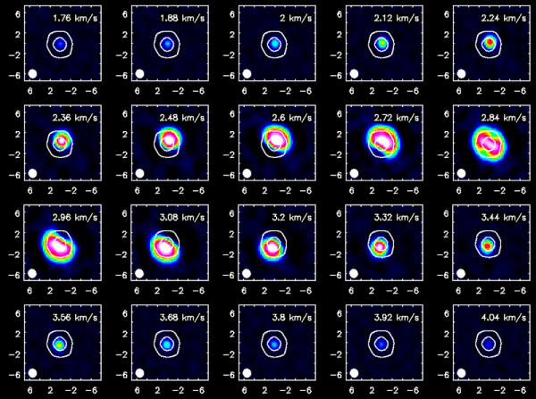
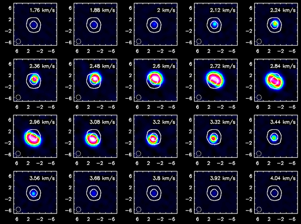
The viewer can be used to make nice figures. In this example we opened the CO(3-2) cube as a raster image and then the continuum as a contour image. Then we used the "wrench" icon and "P wrench" icons to set up the channel images, contour levels etc.

Channel maps of the CO(3-2) emission with white continuum contours at 3 and 100 sigma.

Channel maps of the HCO+(4-3) emission with white continuum contours at 3 and 100 sigma. The color intensity scale is the same as that used for CO(3-2).

Further Image Analysis

To determine channel ranges it is useful to open cube in viewer as a raster. Using the statistics tool the rms in a line free channel is about 25 mJy/beam. Now open the cube again but as a contour map and set the Unit Contour Level to 0.025 (this is in Jy/beam) and in Relative Contour levels set [3]. i.e. this is showing 3sigma contours. Now find out where the CO(3-2) emission drops below the 3sigma level.

For moment 0 (integrated intensity) maps you do not typically want to set a flux threshold because this will tend to noise bias your integrated intensity.

# In CASA
immoments(imagename='TWHydra_CO3_2line.image',moments=[0],
          outfile='TWHydra_CO3_2line.image.mom0',
          chans='40~76')

For higher order moments it is very important to set a conservative flux threshold. Typically something like 10sigma works well.

# In CASA
immoments(imagename='TWHydra_CO3_2line.image',moments=[1,2],
          outfile='TWHydra_CO3_2line.image.mom',
          chans='40~76',includepix=[0.25,100])

ALMA CO(3-2) moment maps, with white continuum contours at 3 and 100 sigma. From left to right: integrated intensity, intensity weighted velocity field, intensity weighted velocity dispersion are shown.

Repeat for HCO+(4-3) which has a bit narrower velocity extent than the CO(3-2), but similar rms noise.

# In CASA
immoments(imagename='TWHydra_CO3_2line.image',moments=[0],
          outfile='TWHydra_CO3_2line.image.mom0',
          chans='43~74')

# In CASA
immoments(imagename='TWHydra_CO3_2line.image',moments=[1,2],
          outfile='TWHydra_CO3_2line.image.mom',
          chans='43~74',includepix=[0.25,100])

ALMA HCO+(4-3) moment maps, with white continuum contours at 3 and 100 sigma. From left to right: integrated intensity, intensity weighted velocity field, intensity weighted velocity dispersion are shown.