Self-Calibration Template CASA 6.1.1: Difference between revisions
| Line 3: | Line 3: | ||
== Self-Calibration on the Continuum (optional) == | == Self-Calibration on the Continuum (optional) == | ||
If you have a high signal-to-noise detection of your source, you can use the source itself to calibrate the phases and potentially the amplitudes of the visibilities as a function of time. This technique is called self-calibration and takes advantage of the fact that interferometer data is over-constrained (we have more equations than we have solutions). | If you have a high signal-to-noise detection of your source, you can use the source itself to calibrate the phases and potentially the amplitudes of the visibilities as a function of time. This technique is called self-calibration and takes advantage of the fact that interferometer data is over-constrained (we have more equations than we have solutions). The recommended signal to noise depends on the number of antennas. As a rule of thumb, [xxx add some recommendations here based on Crystal's self-cal presentation.] | ||
Self-calibration can either be performed with line or continuum data. Here we demonstrate how to do it with continuum data. The principle is the same for line data, except you form your image using the brightest line emission. For an example of self-calibration with line data, see the [[https://casaguides.nrao.edu/index.php?title=VLA_high_frequency_Spectral_Line_tutorial_-_IRC%2B10216#UV_Continuum_Subtraction_and_Setting_Up_for_Self-Calibration | VLA high frequency spectral line tutorial for IRC+10216]. | |||
For a more detailed explanation of self-calibration, please see the NRAO Live! presentation [https://science.nrao.edu/facilities/alma/naasc-workshops/nrao-cd-wm16/Selfcal_Madison.pdf When, why, and how to do self-calibration]. | |||
The first thing you should do when beginning self-calibration is to save the original flags in your data set. This step is necessary because when you apply the calibration to a data set it flags data that is not associated with a solution. Applying a bad calibration table to your data can result in the excessive flagging of your data. | |||
<source lang="python"> | <source lang="python"> | ||
# in CASA | # in CASA | ||
contvis = ' | flagmanager(vis=contvis,mode='save',versionname='before_selfcal',merge='replace') | ||
</source> | </source> | ||
Now we can set up the parameters for the self-cal. Begin by setting the parameters for your ms and continuum image name. The ms '''calibrated_final_cont.ms''' was created in the previous part of this guide: '''[[Image_Continuum | Image the Continuum Template]]'''. | |||
<source lang="python"> | <source lang="python"> | ||
# in CASA | # in CASA | ||
contvis = 'calibrated_final_cont.ms' | |||
contimagename = 'calibrated_final_cont' | |||
</source> | </source> | ||
If you run the self-calibration process more than once, you will need to remove any models that could be left in the image header; which can be accomplished by using the {{delmod}} task as well as the {{clearcal}} task (which will need to be uncommented in the code below). | |||
<source lang="python"> | <source lang="python"> | ||
# in CASA | # in CASA | ||
# delmod(vis=contvis,field=field,otf=True) | |||
# clearcal(vis=contvis) | |||
</source> | </source> | ||
You should use the same reference antenna that was used during calibration. For pipeline reductions, this can be found in the stage '''hif_refant'''. For manual reductions, the reference antenna will be stated near the top of *.ms.scriptForCalibration.py. If there are multiple executions, make sure to use an antenna that has good solutions and is present in all executions. The Analysis Utilities task [https://safe.nrao.edu/wiki/bin/view/ALMA/CommonAntennas au.commonAntennas] can help you find antennas that meet this criteria. Tasks such as {{plotants}} or {{listobs}}/{{vishead}} can also be used to find antennas in all executions. | |||
<source lang="python"> | <source lang="python"> | ||
# in CASA | # in CASA | ||
refant = 'DV09' # pick a reference antenna. | |||
</source> | </source> | ||
In the | In the example below, we combine the signal from all spectral windows to improve the signal-to-noise for our gain solution. When combining the spectral windows, you need to map the solution from the combined spectral window (0) to the individual spectral windows using the spwmap parameter. This parameter is a list where the index of the element in the list indicates the spectral window and the value for that index the window that it is mapped to. For example, if we have three spectral windows in the original data set and use combine='spw' for our gain solution, we set spwmap=[0,0,0] to map spw=0 to spw=0, spw=1 to spw=0, and spw=2 to spw=0. | ||
You then begin the process of shallowly cleaning your continuum | You then begin the process of shallowly cleaning your continuum data to create an initial model for your data in the model column of your data set. Usually you only should do at most a few hundred iterations on the brightest source(s) in the field. | ||
<source lang="python"> | <source lang="python"> | ||
| Line 71: | Line 69: | ||
# Note number of iterations performed. | # Note number of iterations performed. | ||
</source> | |||
Next you take that model and use it to determine the per-antenna phase solutions as a function of time using {{gaincal}}. We use the {{rmtables}} command here to completely eradicate any previous solution table from CASA's memory. Note that we start here with a fairly long solution interface that is the length of a scan (solint='inf'). | |||
<source lang="python"> | |||
# per scan solution | # per scan solution | ||
rmtables('pcal1') | rmtables('pcal1') | ||
| Line 85: | Line 90: | ||
</source> | </source> | ||
Inspect the logging messages output by {{gaincal}} to see how many solutions were expected/attempted/succeeded. If you have a large number of failed solutions, do not proceed further! This usually means that you do not have enough signal-to-noise on your source to proceed with self-calibration. Note that if you apply a calibration table with many failed solutions to the data, it will flag the data associated with these solutions. | |||
<pre style="background-color: #fffacd;"> | <pre style="background-color: #fffacd;"> | ||
| Line 96: | Line 102: | ||
[[File:Plotcal_image.png|thumb|<caption>Solutions from the first round of self-cal.</caption>]] | [[File:Plotcal_image.png|thumb|<caption>Solutions from the first round of self-cal.</caption>]] | ||
</figure> | </figure> | ||
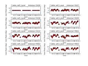
You should also check the solutions (above) that were obtained using {{plotcal}}. | You should also check the solutions (above) that were obtained using {{plotcal}}. The solutions should vary smoothly with time and there should not be any large outliers. | ||
<source lang="python"> | <source lang="python"> | ||
| Line 112: | Line 117: | ||
</source> | </source> | ||
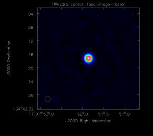
If you are satisfied with the solutions, apply them to the ms and clean the | If you are satisfied with the solutions, apply them to the ms and clean the corrected visibilities. Note that we always want to be generating our model from the latest gaincal solutions, but you should be generating the calibration tables by comparing the original visibilities to the model. This prevents bad solutions from propagating through the self-calibration. | ||
<figure id="Pcal1.png"> | <figure id="Pcal1.png"> | ||
[[File:Pcal1.png|thumb|<caption>Continuum image after the first round of self-cal.</caption>]] | [[File:Pcal1.png|thumb|<caption>Continuum image after the first round of self-cal.</caption>]] | ||
</figure> | </figure> | ||
<source lang="python"> | <source lang="python"> | ||
# in CASA | # in CASA | ||
| Line 127: | Line 134: | ||
flagbackup=False, | flagbackup=False, | ||
interp='linearperobs') | interp='linearperobs') | ||
</source> | |||
With our initial | |||
<source lang="python"> | |||
# clean deeper | # clean deeper | ||
for ext in ['.flux','.image','.mask','.model','.pbcor','.psf','.residual','.flux.pbcoverage']: | for ext in ['.flux','.image','.mask','.model','.pbcor','.psf','.residual','.flux.pbcoverage']: | ||
Revision as of 12:54, 7 May 2017
This guide continues with products created in Image the Continuum Template. All imaging parameters are set in the previous guide. You will need calibrated_final_cont.ms to proceed.
Self-Calibration on the Continuum (optional)
If you have a high signal-to-noise detection of your source, you can use the source itself to calibrate the phases and potentially the amplitudes of the visibilities as a function of time. This technique is called self-calibration and takes advantage of the fact that interferometer data is over-constrained (we have more equations than we have solutions). The recommended signal to noise depends on the number of antennas. As a rule of thumb, [xxx add some recommendations here based on Crystal's self-cal presentation.]
Self-calibration can either be performed with line or continuum data. Here we demonstrate how to do it with continuum data. The principle is the same for line data, except you form your image using the brightest line emission. For an example of self-calibration with line data, see the [| VLA high frequency spectral line tutorial for IRC+10216.
For a more detailed explanation of self-calibration, please see the NRAO Live! presentation When, why, and how to do self-calibration.
The first thing you should do when beginning self-calibration is to save the original flags in your data set. This step is necessary because when you apply the calibration to a data set it flags data that is not associated with a solution. Applying a bad calibration table to your data can result in the excessive flagging of your data.
# in CASA
flagmanager(vis=contvis,mode='save',versionname='before_selfcal',merge='replace')
Now we can set up the parameters for the self-cal. Begin by setting the parameters for your ms and continuum image name. The ms calibrated_final_cont.ms was created in the previous part of this guide: Image the Continuum Template.
# in CASA
contvis = 'calibrated_final_cont.ms'
contimagename = 'calibrated_final_cont'
If you run the self-calibration process more than once, you will need to remove any models that could be left in the image header; which can be accomplished by using the delmod task as well as the clearcal task (which will need to be uncommented in the code below).
# in CASA
# delmod(vis=contvis,field=field,otf=True)
# clearcal(vis=contvis)
You should use the same reference antenna that was used during calibration. For pipeline reductions, this can be found in the stage hif_refant. For manual reductions, the reference antenna will be stated near the top of *.ms.scriptForCalibration.py. If there are multiple executions, make sure to use an antenna that has good solutions and is present in all executions. The Analysis Utilities task au.commonAntennas can help you find antennas that meet this criteria. Tasks such as plotants or listobs/vishead can also be used to find antennas in all executions.
# in CASA
refant = 'DV09' # pick a reference antenna.
In the example below, we combine the signal from all spectral windows to improve the signal-to-noise for our gain solution. When combining the spectral windows, you need to map the solution from the combined spectral window (0) to the individual spectral windows using the spwmap parameter. This parameter is a list where the index of the element in the list indicates the spectral window and the value for that index the window that it is mapped to. For example, if we have three spectral windows in the original data set and use combine='spw' for our gain solution, we set spwmap=[0,0,0] to map spw=0 to spw=0, spw=1 to spw=0, and spw=2 to spw=0.
You then begin the process of shallowly cleaning your continuum data to create an initial model for your data in the model column of your data set. Usually you only should do at most a few hundred iterations on the brightest source(s) in the field.
# in CASA
# shallow clean on the continuum

for ext in ['.flux','.image','.mask','.model','.pbcor','.psf','.residual','.flux.pbcoverage']:
    rmtables(contimagename + '_p0'+ ext)

clean(vis=contvis,
      imagename=contimagename + '_p0',
      field=field,
#      phasecenter=phasecenter, # uncomment if mosaic.
      mode='mfs',
      psfmode='clark',
      imsize = imsize,
      cell= cell,
      weighting = weighting,
      robust=robust,
      niter=niter,
      threshold=threshold,
      interactive=True,
      usescratch=True, # needed for 4.3 and 4.4 (and maybe 4.5)
      imagermode=imagermode)

# Note number of iterations performed.
Next you take that model and use it to determine the per-antenna phase solutions as a function of time using gaincal. We use the rmtables command here to completely eradicate any previous solution table from CASA's memory. Note that we start here with a fairly long solution interface that is the length of a scan (solint='inf').
# per scan solution
rmtables('pcal1')
gaincal(vis=contvis,
        caltable='pcal1',
        field=field,
        gaintype='T',
        refant=refant,
        calmode='p',
        combine='spw',
        solint='inf',
        minsnr=3.0,
        minblperant=6)
Inspect the logging messages output by gaincal to see how many solutions were expected/attempted/succeeded. If you have a large number of failed solutions, do not proceed further! This usually means that you do not have enough signal-to-noise on your source to proceed with self-calibration. Note that if you apply a calibration table with many failed solutions to the data, it will flag the data associated with these solutions.
Calibration solve statistics per spw: (expected/attempted/succeeded):
   Spw 0: 235/235/235
   Spw 1: 235/235/235
   Spw 2: 235/235/235
<figure id="Plotcal_image.png">
</figure>
You should also check the solutions (above) that were obtained using plotcal. The solutions should vary smoothly with time and there should not be any large outliers.
In CASA
# Check the solution
plotcal(caltable='pcal1',
        xaxis='time',
        yaxis='phase',
        timerange='',
        iteration='antenna',
        subplot=421,
        plotrange=[0,0,-180,180])
If you are satisfied with the solutions, apply them to the ms and clean the corrected visibilities. Note that we always want to be generating our model from the latest gaincal solutions, but you should be generating the calibration tables by comparing the original visibilities to the model. This prevents bad solutions from propagating through the self-calibration.
<figure id="Pcal1.png">
</figure>
# in CASA
# apply the calibration to the data for next round of imaging
applycal(vis=contvis,
         field=field,
         spwmap=spwmap,
         gaintable=['pcal1'],
         gainfield='',
         calwt=False,
         flagbackup=False,
         interp='linearperobs')
With our initial
# clean deeper
for ext in ['.flux','.image','.mask','.model','.pbcor','.psf','.residual','.flux.pbcoverage']:
    rmtables(contimagename + '_p1'+ ext)

clean(vis=contvis,
      field=field,
#      phasecenter=phasecenter, # uncomment if mosaic.
      imagename=contimagename + '_p1',
      mode='mfs',
      psfmode='clark',
      imsize = imsize,
      cell= cell,
      weighting = weighting,
      robust=robust,
      niter=niter,
      threshold=threshold,
      interactive=True,
      usescratch=True, # needed for 4.3 and 4.4 (and maybe 4.5)
      imagermode=imagermode)

# Note number of iterations performed.
Inspect the new image in the viewer to see if the first iteration of self-cal worked. Find and compare the new RMS, beam size, and dynamic range of the image to the calibrated_final_cont_p0.image. If the RMS noise increased, do not proceed with the self-calibration. You may try changing the minsnr and minblperant parameters in the gaincal call above to find more solutions. If you are unable to improve the image using self-calibration, undo the self-calibration and skip to the continuum subtraction section of this guide. If the RMS noise and dynamic range improved, proceed with self-calibration below. The next gaincal call uses a shorter solution interval (solint). Continue on with the self-calibration as long as the image statistics continue to improve.
# in CASA
# shorter solution
rmtables('pcal2')
gaincal(vis=contvis,
        field=field,
        caltable='pcal2',
        gaintype='T',
        refant=refant,
        calmode='p',
        combine='spw',
        solint='30.25s', # solint=30.25s gets you five 12m integrations, while solint=50.5s gets you five 7m integration
        minsnr=3.0,
        minblperant=6)

# Check the solution
plotcal(caltable='pcal2',
        xaxis='time',
        yaxis='phase',
        timerange='',
        iteration='antenna',
        subplot=421,
        plotrange=[0,0,-180,180])

# apply the calibration to the data for next round of imaging
applycal(vis=contvis,
         spwmap=spwmap,
         field=field,
         gaintable=['pcal2'],
         gainfield='',
         calwt=False,
         flagbackup=False,
         interp='linearperobs')

# clean deeper
for ext in ['.flux','.image','.mask','.model','.pbcor','.psf','.residual','.flux.pbcoverage']:
    rmtables(contimagename + '_p2'+ ext)

clean(vis=contvis,
      imagename=contimagename + '_p2',
      field=field,
#      phasecenter=phasecenter, # uncomment if mosaic.
      mode='mfs',
      psfmode='clark',
      imsize = imsize,
      cell= cell,
      weighting = weighting,
      robust=robust,
      niter=niter,
      threshold=threshold,
      interactive=True,
      usescratch=True, # needed for 4.3 and 4.4 (and maybe 4.5)
      imagermode=imagermode)

# Note number of iterations performed.

# shorter solution
rmtables('pcal3')
gaincal(vis=contvis,
        field=field,
        caltable='pcal3',
        gaintype='T',
        refant=refant,
        calmode='p',
        combine='spw',
        solint='int',
        minsnr=3.0,
        minblperant=6)

# Check the solution
plotcal(caltable='pcal3',
        xaxis='time',
        yaxis='phase',
        timerange='',
        iteration='antenna',
        subplot=421,
        plotrange=[0,0,-180,180])

# apply the calibration to the data for next round of imaging
applycal(vis=contvis,
         spwmap=spwmap,
         field=field,
         gaintable=['pcal3'],
         gainfield='',
         calwt=False,
         flagbackup=False,
         interp='linearperobs')

for ext in ['.flux','.image','.mask','.model','.pbcor','.psf','.residual','.flux.pbcoverage']:
    rmtables(contimagename + '_p3'+ ext)

clean(vis=contvis,
      imagename=contimagename + '_p3',
      field=field,
#      phasecenter=phasecenter, # uncomment if mosaic.
      mode='mfs',
      psfmode='clark',
      imsize = imsize,
      cell= cell,
      weighting = weighting,
      robust=robust,
      niter=niter,
      threshold=threshold,
      interactive=True,
      usescratch=True, # needed for 4.3 and 4.4 (and maybe 4.5)
      imagermode=imagermode)

# Note number of iterations performed.
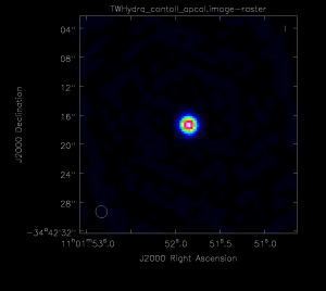
<figure id="Apcal.png">
</figure> The next section performs an amplitude calibration. While the phase calibration involved iterating with different solution intervals, the amplitude self-calibration will only use an infinite solution interval.
# in CASA
rmtables('apcal')
gaincal(vis=contvis,
        field=field,
        caltable='apcal',
        gaintype='T',
        refant=refant,
        calmode='ap',
        combine='spw',
        solint='inf',
        minsnr=3.0,
        minblperant=6,
#        uvrange='>50m', # may need to use to exclude extended emission
        gaintable='pcal3',
        spwmap=spwmap,
        solnorm=True)

plotcal(caltable='apcal',
        xaxis='time',
        yaxis='amp',
        timerange='',
        iteration='antenna',
        subplot=421,
        plotrange=[0,0,0.2,1.8])

applycal(vis=contvis,
         spwmap=[spwmap,spwmap], # select which spws to apply the solutions for each table
         field=field,
         gaintable=['pcal3','apcal'],
         gainfield='',
         calwt=False,
         flagbackup=False,
         interp='linearperobs')

# Make amplitude and phase self-calibrated image.
for ext in ['.flux','.image','.mask','.model','.pbcor','.psf','.residual','.flux.pbcoverage']:
    rmtables(contimagename + '_ap'+ ext)

clean(vis=contvis,
      imagename=contimagename + '_ap',
      field=field,
 #      phasecenter=phasecenter, # uncomment if mosaic.
      mode='mfs',
      psfmode='clark',
      imsize = imsize,
      cell= cell,
      weighting = weighting,
      robust=robust,
      niter=niter,
      threshold=threshold,
      interactive=True,
      usescratch=True, # needed for 4.3 and 4.4 (and maybe 4.5)
      imagermode=imagermode)
Compare all of the images produced during self-calibration. Only apply solutions that continue to improve the image statistics.
The results of the self-cal should be split out via the split command and saved as a *.selfcal file.
# in CASA
split(vis=contvis,
outputvis=contvis+'.selfcal', datacolumn='corrected')
If you are unhappy with the self-calibration, use the clearcal task and restore the original flags to return your ms to it’s original pre-self-cal state.
# in CASA
# uncomment the following to revert to pre self-cal ms
# flagmanager(vis=contvis, mode='restore',versionname='before_selfcal')
# clearcal(contvis)
# delmod(contvis,field=field,otf=True)
You will subtract the continuum and apply the self-calibration results to the line data on the next page, Spectral Line Imaging Template.


