NGC3256 Band3 Imaging for CASA 4.4
Overview
This guide is designed for CASA 4.4. If you are using an older version of CASA please see NGC3256 Band3 Calibration for CASA 4.3.
This portion of the NGC3256Band3 CASA Guide for CASA 4.4 will cover the imaging of the continuum and spectral line data. It begins where the NGC3256 Band3 Calibration for CASA 4.4 section left off: right after running the CASA task split to split off the science target from the rest of the measurement set following calibration. If you completed the Calibration section of the guide, then you can continue where you left off, with ngc3256_line_target.ms. If you did not complete the Calibration portion of the guide, then you can download the calibrated uvdata by clicking on the region closest to your location:
Once there, download the file 'NGC3256_Band3_CalibratedData4.1.tgz' to obtain the calibrated uvdata. The "4.1" in the file name means that the data were processed with an earlier version of CASA but since that version is compatible with CASA 4.4, we have not regenerated the file.
Once the download has finished, unpack the file:
# In a terminal outside CASA
tar -xvzf NGC3256_Band3_CalibratedData4.1.tgz

cd NGC3256_Band3_CalibratedData

# Start CASA
casapy
After that, you should have ngc3256_line_target.ms in your working directory.
Continuum image of the galaxy
We will start by making a continuum image of the galaxy using clean. Since this dataset contains spectral line emission from both CO and CN, we are careful to select only the channels that are free of line emission. These line-free channels are found by plotting the average amplitudes as a function of channel for each spectral window individually. You will find a strong CO(1-0) emission line in spw 0 in channels 55 to 69, and CN emission lines in spw 1 between channels 35~47 and channels 59~68. You will also find an increased noise level at the very lowest channels.

# In CASA
plotms(vis='ngc3256_line_target.ms',spw='',xaxis='channel',yaxis='amp',
      avgtime='1e8',avgscan=T,iteraxis='spw')
Before starting the cleaning, it makes sense to check if the continuum emission is resolved or not by plotting amplitude as a function of uv-distance. We just plot spw 2 here, because we know that this spectral window is free from line emission.

# In CASA
plotms(vis='ngc3256_line_target.ms',spw='2',xaxis='uvdist',yaxis='amp',
      avgtime='1e8',avgchannel='128',coloraxis='baseline')
For the cleaning we select a spatial mask that just includes the extent of the continuum emission. Here, we use the default non-interactive mode, but if you want to define the clean boxes more carefully, specify interactive=True. In that case, the clean task will bring up a viewer where the clean region can be defined, either by selecting boxes or by selecting polygon regions.
In the configuration that was used, the resolution in Band 3 is approximately 6 arcsec. We therefore choose a cell size of 1 arcsec, so as to oversample the beam sufficiently. The FWHM of the primary beam of ALMA in Band 3 is about 60 arcsec, and we want to image at least that extent. To be on the generous side, we choose to use 100 pixels.
Finally, note that we delete any previous versions of the output images before proceeding with the clean command. This is an important step, because if images with the supplied root name already exist, CASA will clean those further instead of producing new output images.
# In CASA
os.system('rm -rf result-ngc3256_cont*')
clean( vis='ngc3256_line_target.ms', imagename='result-ngc3256_cont',
	spw='0:20~53;71~120,1:70~120,2:20~120,3:20~120', psfmode='hogbom',
	mode='mfs', niter=500, threshold='0.3mJy', mask=[42,43,59,60],
	imsize=100, cell='1arcsec', weighting='briggs', robust=0.0,
	interactive=False, usescratch=False)
The input parameters include:
- vis='ngc3256_line_target.ms': The calibrated dataset on the science target
- imagename='result-ngc3256_cont': The base name of the output images
- spw='0:20~53;71~120,1:70~120,2:20~120,3:20~120': To specify only the channels in each spw free of line emission
- psfmode='hogbom': The method used to calculated the PSF during minor clean cycles. Hogbom is a good choice for poorly-sampled uv-planes
- mode='mfs': Multi-Frequency Synthesis: The default mode, which produces one image from all the specified data combined
- niter=500: Maximum number of clean iterations
- theshold='0.3mJy': Stop cleaning if the maximum residual is below this value. We choose the threshold to be ~1.5 times the rms noise in the image
- mask=[42,43,59,60]: Limits the clean component placement to the region of the source
- imsize=100, cell='1arcsec': Chosen to appropriately sample the resolution element and cover the primary beam
- weighting='briggs', robust=0.0: a weighting scheme that offers a good compromise between sensitivity and resolution
Note the parameter "usescratch" which was introduced in CASA 3.4. It determines whether the model information for later selfcal is explicitly stored in a MODEL_DATA column of the MS (usescratch=True) or if a rule for the creation of the model information on-demand in memory is stored in the MS header (usescratch=False, the default). The latter saves 30 % of disk space and much disk I/O.

We will determine some statistics for the image using the task imstat:
# In CASA
calstat=imstat(imagename='result-ngc3256_cont.image', region='', box='10,10,90,35')
rms=(calstat['rms'][0])
print '>> rms in continuum image: '+str(rms)
calstat=imstat(imagename='result-ngc3256_cont.image', region='')
peak=(calstat['max'][0])
print '>> Peak in continuum image: '+str(peak)
print '>> Dynamic range in continuum image: '+str(peak/rms)
This tells us that the peak flux density of the image is ~7 mJy and the dynamic range is approximately 22. For future reference, we create a png file of the continuum image:
# In CASA
imview(raster={'file': 'result-ngc3256_cont.image', 'colorwedge':T,
        'range':[-0.001, 0.009], 'scaling':0, 'colormap':'Rainbow 2'},
        out='result-ngc3256_cont.png', zoom=2)
Self-Calibration
The continuum flux is fairly low in this galaxy, but given the large bandwidth of ALMA, we have sufficient signal-to-noise to attempt to self-calibrate the data. We will therefore do some phase-only self-calibration of the image using the task gaincal. This will compare the DATA column with the MODEL column, which has been filled with the clean components from the recent run of clean. We use a solution interval of 30 minutes, as we found that this gives just sufficient signal to noise per baseline. Using the ALMA sensitivity calculator, we estimate that the rms noise level per baseline for 30 min integration time and a total bandwidth of 5.1 GHz (excluding the emission lines) is 0.7 mJy. Compared to the peak flux of ~7 mJy, this should give us a sufficient SNR, taking into account that the emission is slightly resolved.
# In CASA
gaincal(vis='ngc3256_line_target.ms', field='NGC*',
    	caltable='cal-ngc3256_cont_30m.Gp',
    	spw='0:20~53;71~120,1:70~120,2:20~120,3:20~120',
    	solint='1800s', refant='DV07', calmode='p',
    	minblperant=3)
- caltable='cal-ngc3256_cont_900.Gp': The name of the output calibration table
- spw='0:20~53;71~120,1:70~120,2:20~120,3:20~120': To select only the continuum channels
- solint='1800s': To specify a 30-minute solution interval
- refant='DV07': Our reference antenna
- calmode='p': To select phase-only solutions
- minblperant=3: To set the minimum number of baselines to other antennas that must be present for a given antenna to have a solution
We then examine the derived phase solutions using plotcal:

# In CASA
plotcal(caltable = 'cal-ngc3256_cont_30m.Gp', xaxis = 'time', yaxis =
	'phase', poln='X', plotsymbol='o', plotrange = [0,0,-180,180],
	iteration = 'spw', figfile='cal-phase_vs_time_XX_30_Gp.png',
	subplot = 221)
# In CASA
plotcal(caltable = 'cal-ngc3256_cont_30m.Gp', xaxis = 'time', yaxis =
	'phase', poln='Y', plotsymbol='o', plotrange = [0,0,-180,180],
	iteration = 'spw', figfile='cal-phase_vs_time_YY_30_Gp.png',
	subplot = 221)
It is also possible to connect the points in a plot by using plotsymbol=":". The phase-only self-cal solutions look good, so we will apply them to the data with applycal. This will overwrite the data in the CORRECTED data column.
# In CASA
applycal(vis='ngc3256_line_target.ms', interp='linear',
	gaintable='cal-ngc3256_cont_30m.Gp')
We then make another continuum map from the newly-corrected data, using the same clean parameters as before.
# In CASA
os.system('rm -rf result-ngc3256_cont_sc1*')
clean( vis='ngc3256_line_target.ms', imagename='result-ngc3256_cont_sc1',
	spw='0:20~53;71~120,1:70~120,2:20~120,3:20~120', psfmode='hogbom',
	mode='mfs', niter=500, threshold='0.13mJy', mask=[42,43,59,60],
        imsize=100, cell='1arcsec', weighting='briggs', robust=0.0,
        interactive=False, usescratch=False)

and again generate some statistics:
# In CASA
calstat=imstat(imagename='result-ngc3256_cont_sc1.image', region='',
box='10,10,90,35')
rms=(calstat['rms'][0])
print '>> rms in continuum image: '+str(rms)
calstat=imstat(imagename='result-ngc3256_cont_sc1.image', region='')
peak=(calstat['max'][0])
print '>> Peak in continuum image: '+str(peak)
print '>> Dynamic range in continuum image: '+str(peak/rms)
The continuum image has improved a lot. The dynamic range is now ~126, whereas before it was only ~22. The image peak flux density is ~10 mJy. We will write this new image to the file 'result-ngc3256_cont_sc1.image' to indicate that an iteration of self-calibration was performed. We also create a new png file of the self-calibrated continuum image.
# In CASA
imview(raster={'file': 'result-ngc3256_cont_sc1.image', 'colorwedge':T,
        'range':[-0.001, 0.010], 'scaling':0, 'colormap':'Rainbow 2'},
        out='result-ngc3256_cont_sc1.png', zoom=2)
In principle, one could experiment further with self-calibration, changing the solution interval, or even adding amplitude self-calibration. To do this, just repeat the steps 1) gaincal, 2) applycal, and 3) clean until you are happy with the result. For the moment, we are happy with just one round of phase-only self-cal.
Line cubes of the galaxy
Before making cubes of the line emission of NGC 3256, we want to subtract the continuum emission from the spectral line data using the task uvcontsub. This task makes fits to the line free channels and subtracts the emission in the uv-domain. It will operate on the CORRECTED_DATA column and will write the continuum subtracted data to a new measurement set with the extension ".contsub". Remember that in the previous section we applied the self-calibration tables to the DATA column to generate this CORRECTED_DATA column.
# In CASA
uvcontsub(vis = 'ngc3256_line_target.ms',
	  fitspw='0:20~53;71~120,1:70~120,2:20~120,3:20~120', solint ='int',
	  fitorder = 1,
	  combine='spw')
- fitspw='0:20~53;71~120,1:70~120,2:20~120,3:20~120': To specify the spectral windows and channels to be used in the fit for the continuum. We avoid the spectral regions that include the CO and CN emission lines.
- solint ='int': Timescale for the per-baseline fit. Here we are electing to have one fit per integration
- fitorder = 1: We will fit a first-order polynomial to the continuum
- combine='spw': Combine spws to form a spw-merged continuum estimate
Next, we will clean the CO (1-0) line emission:
# In CASA
os.system('rm -rf result-ngc3256_line_CO.*')
clean(vis='ngc3256_line_target.ms.contsub', imagename='result-ngc3256_line_CO',
	spw='0:38~87', mode='channel', start='', nchan=-1, width='',
        psfmode='hogbom', outframe='LSRK', restfreq='115.271201800GHz',
        mask=[53,50,87,83], niter=500, interactive=T, imsize=128, cell='1arcsec',
        weighting='briggs', robust=0.0, threshold='5mJy',
        usescratch=False)

Notable parameters include:
- spw='0:38~87': To specify the CO (1-0) line emission alone
- mode='channel': To produce an image with different planes specified by the "start", "nchan", and "width" parameters
- start='', nchan=-1, width='': To include all 50 channels specified by spw, with no channel averaging
- threshold='5 mJy': Stop cleaning if the maximum residual is below this value.
- outframe='LSRK': Shift the output reference frame to the local standard of rest
- restfreq='115.271201800GHz': The rest frequency of the CO line
- mask=[53,50,87,83]: The region in which to fit clean components (i.e., the source)
- niter=500: Maximum number of clean iterations
- interactive=T: To do interactive cleaning with the viewer GUI
- psfmode='hogbom': The method used to calculated the PSF during minor clean cycles. Hogbom is a good choice for poorly-sample uv-planes
Note that you can also find the frequencies of many spectral lines inside CASA. For example, the following commands will search for CO emission lines in ALMA band 3, and output the results to the logger:
# In CASA
os.system('rm -rf myresults.tbl')
slsearch(outfile='myresults.tbl', freqrange = [84,116], species=['COv=0'])
sl.open('myresults.tbl')
sl.list()
Or define the parameter restfreq directly using:
# In CASA
tb.open('myresults.tbl')
restfreq=tb.getcol('FREQUENCY')[0]
tb.close()
Using interactive=T the viewer will open when it is ready to start an interactive clean. Step through to the channels to see how extended the emission is. Then either use "All Channels" to define the same clean mask for all channels, or select "This Channel" to select different masks for each channel. Once you have defined a polygon region, you need to double click inside it to save the mask region. You can use the "tape deck" to step through the channels again and check that the emission in all channels fits within the mask(s) you have created. Note that the mask we defined above does not include all emission -- you will have to change the mask interactively! To continue with clean use the "Next action" buttons in the green area on the Viewer Display GUI: The red X will stop clean where you are; the blue arrow will stop the interactive part of clean, but continue to clean non-interactively until reaching the stopping niter or threshold (whichever comes first); and the green arrow will clean until it reaches the "iterations" parameter on the left side of the green area.
When the cleaning has finished, you may want to inspect the resulting cube and and use the tape deck to play the cube as a movie. Use Spectral Profile in the Tools tab to make an integrated spectrum of the CO(1-0) emission.
# In CASA
imview('result-ngc3256_line_CO.image')
The rms noise level in the cube is ~1 mJy per channel in the line-free channels. The ALMA sensitivity calculator gives a noise level of 0.80 mJy using 7 antennas, an integration time of 3.5 hours, and a bandwidth of 32.25 MHz (this is twice the channel separation because on-line Hanning smoothing was applied.)
Next, we make the moment maps of the CO (1-0) emission using the task immoments:
# In CASA
os.system('rm -rf result-ngc3256_CO1-0.mom0*')
immoments(imagename='result-ngc3256_line_CO.image', moments=[0],
	chans='15~34', box='38,38,90,90', axis='spectral',
	includepix=[0.02, 10000], outfile='result-ngc3256_CO1-0.mom0')
# In CASA
os.system('rm -rf result-ngc3256_CO1-0.mom1*')
immoments(imagename='result-ngc3256_line_CO.image', moments=[1],
	chans='15~34', box='38,38,90,90', axis='spectral',
	includepix=[0.045, 10000], outfile='result-ngc3256_CO1-0.mom1')


- moments=[x]: To specify that we wish to make the xth moment map. The 0th moment map gives integrated emission and the 1st gives the intensity-weighted velocity field
- chans='15~34': These are the channels that show line emission and therefore the ones we want to use for the moment map
- box='38,38,90,90': To select a box region around the emission so as to not include any regions away from the galaxy
- axis='spectral': Indicates the moment axis; in this case, 'spectral'
- includepix=[0.045, 10000]: To select which pixel values in the cube to include in the moments. We find these values by looking for the faintest believable emission in the cube
- outfile='result-ngc3256_CO1-0.mom0': The output image name
Here, we have chosen to run the immoments separately for the total intensity map and the velocity field because we want to use different thresholds for flux inclusion. To find the lower limit in includepix, open the cube in the viewer, and identify the lowest believable flux levels in the cube.
We also make a velocity dispersion map of the CO(1-0) gas, using moments=[2]
# In CASA
os.system('rm -rf result-ngc3256_CO1-0.mom2*')
immoments(imagename='result-ngc3256_line_CO.image', moments=[2],
	chans='5~44', box='38,38,90,90', axis='spectral',
	includepix=[0.035, 10000], outfile='result-ngc3256_CO1-0.mom2')
Now we can make images of the CO(1-0) emission. First create a colour image of the velocity field, with contours of the total line emission overlaid:
# In CASA
imview(contour={'file': 'result-ngc3256_CO1-0.mom0','levels':
       [5,10,20,40,80,160],'base':0,'unit':1},
       raster={'file': 'result-ngc3256_CO1-0.mom1','range': [2630,2920],
       'colorwedge':T, 'colormap': 'Rainbow 2'}, out='result-CO_velfield.png')
Or, make a colour image of the integrated CO(1-0) line emission, with contours of the velocity field overlaid:
# In CASA
imview(contour={'file': 'result-ngc3256_CO1-0.mom1','levels':
        [2650,2700,2750,2800,2850,2900],'base':0,'unit':1},
        raster={'file': 'result-ngc3256_CO1-0.mom0', 'colorwedge':T,
        'colormap': 'Rainbow 2','scaling':-1.0,'range': [0.8,250]},
        out='result-CO_map.png')
And make a greyscale image of the CO(1-0) gas velocity dispersion
# In CASA
imview(contour={'file': 'result-ngc3256_CO1-0.mom2','levels':
        [20,30,40,50,60],'base':0,'unit':1},
        raster={'file': 'result-ngc3256_CO1-0.mom2', 'colorwedge':T,
        'colormap': 'Greyscale 1','scaling':-1.0,'range': [0,74]},
        out='result-CO_dispersion.png')

Also, using the viewer, it is possible to make channel maps. The following image shows six velocity channels, with contours indicating the 3mm continuum emission.
Next, we clean the CN line emission. There are two CN lines, the N=1-0, J=3/2-1/2 line at higher frequency and the N=1-0, J=1/2-1/2 line at lower frequency. We start with the higher frequency line emission. Again, we have set a mask here, but the best results are obtained if an interactive clean mask is defined.
# In CASA
os.system('rm -rf result-ngc3256_line_CNhi.*')
clean(vis='ngc3256_line_target.ms', imagename='result-ngc3256_line_CNhi',
	outframe='LSRK', spw='1:50~76', start='', nchan=27, width='',
	restfreq='113.48812GHz', selectdata=T, mode='channel',
	niter=500, gain=0.1, psfmode='hogbom', mask=[53,50,87,83],
	interactive=True, imsize=128, cell='1arcsec',
	weighting='briggs', robust=0.0, threshold='2mJy',
	usescratch=False)
Make the moment maps of the higher frequency CN line emission:
# In CASA
os.system('rm -rf result-ngc3256_CNhi.mom.*')
immoments( imagename='result-ngc3256_line_CNhi.image', moments=[0,1],
	chans='5~18', axis='spectral', box='38,38,90,90',
	includepix=[0.005, 10000], outfile='result-ngc3256_CNhi.mom')
Make images of the higher frequency CN line emission:
# In CASA
imview(contour={'file': 'result-ngc3256_CNhi.mom.integrated','range': []},
        raster={'file': 'result-ngc3256_CNhi.mom.weighted_coord',
        'range': [2630,2920],'colorwedge':T,
        'colormap': 'Rainbow 2'}, out='result-CNhi_velfield.png')
# In CASA
imview(contour={'file': 'result-ngc3256_CNhi.mom.weighted_coord','levels':
       [2650,2700,2750,2800,2850,2900],'base':0,'unit':1},
       raster={'file': 'result-ngc3256_CNhi.mom.integrated','colorwedge':T,
       'colormap': 'Rainbow 2'}, out='result-CNhi_map.png')
And finally, clean the CN (N=1-0, J=1/2-1/2) emission:
# In CASA
os.system('rm -rf result-ngc3256_line_CNlo.*')
clean( vis='ngc3256_line_target.ms', imagename='result-ngc3256_line_CNlo',
	outframe='LSRK', spw='1:29~54', start='', nchan=26, width='',
	restfreq='113.17049GHz', selectdata=T, mode='channel',
	niter=300, gain=0.1, psfmode='hogbom', mask=[53,50,87,83],
	interactive=True, imsize=128, cell='1arcsec',
	weighting='briggs', robust=0.0, threshold='2mJy',
	usescratch=False)
Make the moment maps of the lower frequency CN emission
# In CASA
os.system('rm -rf result-ngc3256_CNlo.mom.*')
immoments( imagename='result-ngc3256_line_CNlo.image', moments=[0,1],
	chans='8~18', axis='spectral', box='38,38,90,90',
	includepix=[0.003, 10000], outfile='result-ngc3256_CNlo.mom')
Make images of the low frequency CN emission
# In CASA
imview(contour={'file': 'result-ngc3256_CNlo.mom.integrated','range': []},
        raster={'file': 'result-ngc3256_CNlo.mom.weighted_coord',
        'range': [2630,2920],'colorwedge':T,
        'colormap': 'Rainbow 2'}, out='result-CNlo_velfield.png')
# In CASA
imview(contour={'file': 'result-ngc3256_CNlo.mom.weighted_coord','levels':
        [2650,2700,2750,2800,2850,2900],'base':0,'unit':1},
        raster={'file': 'result-ngc3256_CNlo.mom.integrated','colorwedge':T,
        'colormap': 'Rainbow 2'}, out='result-CNlo_map.png')
Note that with 'out' set, imview will just create the image file. It will not open an interactive viewer.
This composite shows the CN maps and velocity fields.
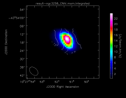
The higher frequency CN(1-0) "moment 0" total intensity maps of NGC3256, with contours of the velocity field overlaid
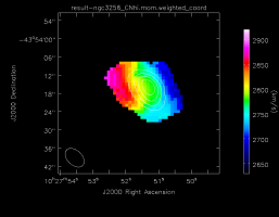
The higher frequency CN(1-0) velocity field of NGC3256, with contours of the total line emission map overlaid

The lower frequency CN(1-0) "moment 0" total intensity maps of NGC3256, with contours of the velocity field overlaid
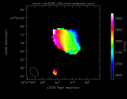
The lower frequency CN(1-0) velocity field of NGC3256, with contours of the total line emission map overlaid


And finally we show the channel maps of all three emission lines overlaid. The 'hot metal' colours represent the higher frequency CN line, the green contours are the CO line, and the cyan contours are the lower frequency CN line.

Last checked on CASA Version 4.4.0.