|
|
| (204 intermediate revisions by 6 users not shown) |
| Line 1: |
Line 1: |
| ==Overview==
| | [[Category:ALMA]][[Category:Calibration]][[Category:Spectral Line]] |
| [To be written by Eric] | |
|
| |
|
| ==Retrieving the Data== | | ==Science Target Overview== |
| | [[File:OpticalImageNGC3256.jpg|200px|thumb|right|HST image of NGC3256 (credit: NASA, ESA, the Hubble Heritage Team (STScI/AURA)-ESA/Hubble Collaboration and A. Evans (University of Virginia, Charlottesville/NRAO/Stony Brook University)]] |
| | [[File:CO2-1_image_SMA.jpg|200px|thumb|right|SMA map of CO (2–1) emission in the center of NGC 3256 (Sakamoto, Ho & Peck, 2006)]] |
|
| |
|
| The data were taken in six different datasets over two consecutive nights: April 16-17, 2011. There are three datasets for April 16th and three for April 17th. Here we provide you with "starter" datasets, where we have taken the raw data in ALMA Science Data Model (ASDM) format and converted them to CASA Measurement Sets (MS). We did this using the {{importasdm}} task in CASA. | | The luminous infrared galaxy NGC 3256 is the brightest galaxy within ~40 Mpc. This galaxy, which is in the later stages of a merger between two gas-rich progenitors, hosts an extreme central starburst that can be seen across a wide range of wavelengths but emits most strongly in the far infrared (Smith & Harvey 1996). Hubble Space Telescope optical imaging has revealed hundreds of bright young clusters in the galactic center (Trancho et al. 2007). There is also strong evidence for a superwind in NGC 3256, indicating strong starburst-driven blow-out of the interstellar medium (Heckman et al. 2000). Imaging in the infrared, radio and X-rays has shown that NGC 3256 has two distinct nuclei aligned in the north-south direction and separated by 5 arcsec, or 850 pc, on the sky. The southern nucleus is highly obscured, rendering it invisible in the optical. |
|
| |
|
| [What else are we going to do to the data we provide?]
| | Because of its proximity and the fact that it is observed nearly face-on, NGC 3256 is an ideal target to study merger-induced starbursts in the local Universe. In fact, NGC 3256 could be regarded as the southern sky equivalent of Arp 220, the archetype of infrared-luminous merging galaxies. |
|
| |
|
| Along with the Measurement Sets, we also provide some tables that you will need for the calibration. These include the System Temperature (Tsys) tables, which contain corrections for atmospheric opacity, and Water Vapor Radiometer (WVR) tables, which contain the atmospheric phase corrections determined by the water vapor radiometers on each antenna.
| | Neutral gas in this galaxy was first studied by English et al (2003), who detected two HI tidal tails that extend up to 50 kpc. High-resolution observations of carbon-monoxide (CO 2-1) in NGC 3256 were made by Sakamoto et al. (2006) using the Submillimeter Array (SMA). This study revealed a large disk of molecular gas (r > 3 kpc) in the center of the merger, with a strong gas concentration toward the double nucleus. This gas disk rotates around a point between the two nuclei. In addition, high-velocity molecular gas was discovered at the galaxy's center, with velocities up to 420 km/s offset from the systemic velocity of the galaxy. |
|
| |
|
| You can download the data here:
| | ==ALMA Data Overview== |
| [Provide link to the raw .ms files in tar'd, gzip'd format]
| | ALMA Science verification data on NGC3256 in Band 3 were taken in six different |
| | datasets over two consecutive nights: April 16-17, 2011. There are three datasets |
| | for April 16th and three for April 17th. These Band 3 observations utilized all four |
| | available basebands, which are associated with four different spectral windows: two |
| | in the Upper Sideband (USB) and two in the Lower Sideband (LSB). The first spectral |
| | window is centered on the CO(1-0) emission line in the galaxy NGC 3256 and is our |
| | highest frequency spectral window. There is one additional spectral window in the |
| | Upper Side Band (USB), and there are two spectral windows in the Lower Side Band |
| | (LSB). These additional spectral windows are used to measure the continuum emission |
| | in the galaxy and may contain other emission lines as well. Each spectral window |
| | has a total bandwidth of 2 GHz divided over 128 channels, for a channel width of |
| | 15.625 MHz, corresponding to about 40 km/s. Online Hanning smoothing was applied to |
| | the data, resulting in a spectral resolution that is twice the channel separation. |
| | For the antenna configuration that was used during these observations, the angular |
| | resolution is expected to be about 6.5". |
|
| |
|
| Once the download has finished, unpack the file:
| | Due to unfortunate weather conditions during the days planned for these |
| <source lang="python">
| | observations, the data were taken at Band 3 although no previous interferometric |
| # In a terminal outside CASA
| | CO(1-0) observations of this galaxy exist. Casoli et al. (1990) observed the CO(1-0) |
| tar -xvf ngc3256band3.tgz
| | line with the SEST 15 single dish telescope and were just able to measure a velocity |
| </source>
| | field with 22" resolution. Interferometric observations were first made with the SMA |
| | in the CO(2-1) line by Sakamoto, Ho & Peck (2006). Because those observations were |
| | made at a higher frequency, the angular resolution is higher (~2") than that of the |
| | ALMA observations shown here, taken in a very compact configuration. Nonetheless, it |
| | is possible to make a direct comparison of the distribution and velocity of the |
| | CO(2-1) and (1-0) gas by looking, for example, at the south-western clump and the |
| | north-eastern 'arm', which are consistent in both data sets. |
|
| |
|
| [Also provide links to the calibrated data (but maybe not here...maybe better at end of calibration page?)]
| | We thank the following people for suggesting NGC3256 for ALMA Science Verification: |
| | Kazushi Sakamoto, Satoki Matsushita. |
|
| |
|
| ==Initial Inspection and ''A priori '' Flagging== | | ==Obtaining the Data== |
| We will eventually concatenate the six datasets used here into one large dataset. However, we will keep them separate for now, as some of the steps to follow require individual datasets (specifically, the application of the Tsys and WVR tables). We therefore start by defining an array 'basename' that includes the names of the six files. This will simplify the following steps by allowing us to loop through the files using a simple for-loop in python.
| |
|
| |
|
| <source lang="python">
| | To download the data, click on the region closest to your location: |
| # In CASA
| |
| basename=['uid___A002_X1d54a1_X5','uid___A002_X1d54a1_X174','uid___A002_X1d54a1_X2e3','uid___A002_X1d5a20_X5','uid___A002_X1d5a20_X174','uid___A002_X1d5a20_X330']
| |
| </source>
| |
|
| |
|
| The usual first step is then to get some basic information about the data. We do this using the task {{listobs}}, which will output a detailed summary of each dataset supplied.
| | [http://almascience.nrao.edu/almadata/sciver/NGC3256 North America] |
|
| |
|
| <source lang="python">
| | [http://almascience.eso.org/almadata/sciver/NGC3256 Europe] |
| # In CASA
| |
| for name in basename:
| |
| listobs(vis=name+'.ms')
| |
| </source>
| |
|
| |
|
| The output will be sent to the CASA logger. You will have to scroll up to see the individual output for each of the six datasets. Here is an example of the most relevant output for the first file in the list.
| | [http://almascience.nao.ac.jp/almadata/sciver/NGC3256 East Asia] |
|
| |
|
| <pre style="background-color: #fffacd;">
| | Here you will find three gzipped tar files which, after unpacking, will create three directories: |
| Fields: 3
| |
| ID Code Name RA Decl Epoch SrcId nVis
| |
| 0 none 1037-295 10:37:16.0790 -29.34.02.8130 J2000 0 38759
| |
| 1 none Titan 00:00:00.0000 +00.00.00.0000 J2000 1 16016
| |
| 2 none NGC3256 10:27:51.6000 -43.54.18.0000 J2000 2 151249
| |
| (nVis = Total number of time/baseline visibilities per field)
| |
| Spectral Windows: (9 unique spectral windows and 2 unique polarization setups)
| |
| SpwID #Chans Frame Ch1(MHz) ChanWid(kHz)TotBW(kHz) Ref(MHz) Corrs
| |
| 0 4 TOPO 184550 1500000 7500000 183300 I
| |
| 1 128 TOPO 113211.988 15625 2000000 113204.175 XX YY
| |
| 2 1 TOPO 114188.55 1796875 1796875 113204.175 XX YY
| |
| 3 128 TOPO 111450.813 15625 2000000 111443 XX YY
| |
| 4 1 TOPO 112427.375 1796875 1796875 111443 XX YY
| |
| 5 128 TOPO 101506.187 15625 2000000 101514 XX YY
| |
| 6 1 TOPO 100498.375 1796875 1796875 101514 XX YY
| |
| 7 128 TOPO 103050.863 15625 2000000 103058.675 XX YY
| |
| 8 1 TOPO 102043.05 1796875 1796875 103058.675 XX YY
| |
| Sources: 48
| |
| ID Name SpwId RestFreq(MHz) SysVel(km/s)
| |
| 0 1037-295 0 - -
| |
| 0 1037-295 9 - -
| |
| 0 1037-295 10 - -
| |
| 0 1037-295 11 - -
| |
| 0 1037-295 12 - -
| |
| 0 1037-295 13 - -
| |
| 0 1037-295 14 - -
| |
| 0 1037-295 15 - -
| |
| 0 1037-295 1 - -
| |
| 0 1037-295 2 - -
| |
| 0 1037-295 3 - -
| |
| 0 1037-295 4 - -
| |
| 0 1037-295 5 - -
| |
| 0 1037-295 6 - -
| |
| 0 1037-295 7 - -
| |
| 0 1037-295 8 - -
| |
| 1 Titan 0 - -
| |
| 1 Titan 9 - -
| |
| 1 Titan 10 - -
| |
| 1 Titan 11 - -
| |
| 1 Titan 12 - -
| |
| 1 Titan 13 - -
| |
| 1 Titan 14 - -
| |
| 1 Titan 15 - -
| |
| 1 Titan 1 - -
| |
| 1 Titan 2 - -
| |
| 1 Titan 3 - -
| |
| 1 Titan 4 - -
| |
| 1 Titan 5 - -
| |
| 1 Titan 6 - -
| |
| 1 Titan 7 - -
| |
| 1 Titan 8 - -
| |
| 2 NGC3256 0 - -
| |
| 2 NGC3256 9 - -
| |
| 2 NGC3256 10 - -
| |
| 2 NGC3256 11 - -
| |
| 2 NGC3256 12 - -
| |
| 2 NGC3256 13 - -
| |
| 2 NGC3256 14 - -
| |
| 2 NGC3256 15 - -
| |
| 2 NGC3256 1 - -
| |
| 2 NGC3256 2 - -
| |
| 2 NGC3256 3 - -
| |
| 2 NGC3256 4 - -
| |
| 2 NGC3256 5 - -
| |
| 2 NGC3256 6 - -
| |
| 2 NGC3256 7 - -
| |
| 2 NGC3256 8 - -
| |
| Antennas: 7:
| |
| ID Name Station Diam. Long. Lat.
| |
| 0 DV04 J505 12.0 m -067.45.18.0 -22.53.22.8
| |
| 1 DV06 T704 12.0 m -067.45.16.2 -22.53.22.1
| |
| 2 DV07 J510 12.0 m -067.45.17.8 -22.53.23.5
| |
| 3 DV08 T703 12.0 m -067.45.16.2 -22.53.23.9
| |
| 4 DV09 N602 12.0 m -067.45.17.4 -22.53.22.3
| |
| 5 PM02 T701 12.0 m -067.45.18.8 -22.53.22.2
| |
| 6 PM03 J504 12.0 m -067.45.17.0 -22.53.23.0
| |
| </pre>
| |
|
| |
|
| This output shows that three fields were observed: 1037-295, Titan, and NGC3256. Field 0 (1037-295) will serve as the gain calibrator and bandpass calibrator; field 1 (Titan) will serve as the flux calibrator; and field 2 (NGC3256) is, of course, the science target.
| | *'''NGC3256_Band3_UnCalibratedMSandTablesForReduction''' - Here we provide you with "starter" datasets, where we have taken the raw data in ALMA Science Data Model (ASDM) format and converted them to CASA Measurement Sets (MS). We did this using the {{importasdm}} task in CASA. Along with the raw data, we also provide some tables that you will need for the calibration which cannot currently be generated inside of CASA (for Early Science, these tables will either be pre-applied or supplied with the data). |
|
| |
|
| Note that there are more than four SpwIDs even though the observations were set up to have four spectral windows. The spectral line data themselves are found in spectral windows 1,3,5,7, which have 128 channels each. The first one (spw 1) is centered on the CO(1-0) emission line in the galaxy NGC 3256 and is our highest frequency spectral window. There is one additional spectral window (spw 3) in the Upper Side Band (USB), and there are two spectral windows (spw 5 and 7) in the Lower Side Band (LSB). These additional spectral windows are used to measure the continuum emission in the galaxy, and may contain other emission lines as well.
| | *'''NGC3256_Band3_CalibratedData''' - The fully-calibrated uvdata, ready for imaging and self-calibration |
|
| |
|
| Spectral windows 2,4,6,8 contain channel averages of the data in spectral windows 1,3,5,7, respectively. These are not useful for the offline data reduction. Spectral window 0 contains the WVR data. You may notice that there are additional SpwIDs listed in the "Sources" section which are not listed in the "Spectral Windows" section. These spectral windows are reserved for the WVRs of each antenna (seven in our case). At the moment, all WVRs point to spw 0, which contains nominal frequencies. The additional spectral windows (spw 9-15) are therefore not used and can be ignored.
| | *'''NGC3256_Band3_ReferenceImages''' - The final continuum and spectral line images |
|
| |
|
| Another important thing to note is that the position of Titan is listed as 00:00:00.0000 +00.00.00.0000. This is due to the fact that for ephemeris objects, the positions are currently not stored in the asdm. This will be handled correctly in the near future, but at present, we have to fix this offline. We will correct the coordinates below by running the procedure fixplanet.
| | To see which files you will need, read on below. The downloads to your local computer will take some time, so you may wish to begin them now. |
|
| |
|
| There were seven antennas in the array for these observations. Note that numbering in python always begins with "0", so the antennas have IDs 0-6. To see what the antenna configuration looked like at the time of the observations, we will use the task {{plotants}}. Since the configuration did not change during the course of the observations, we will simply look at the first dataset from the list.
| | '''NOTE: CASA 3.3 or later is required to follow this guide.''' For more information on obtaining the latest version of CASA, see [http://casa.nrao.edu/ http://casa.nrao.edu]. |
|
| |
|
| <source lang="python">
| | ==NGC3256 Data Reduction Tutorial== |
| # In CASA
| |
| plotants(vis=basename[0]+'.ms', figfile='ngc3256band3_plotants.png')
| |
| </source>
| |
|
| |
|
| This will plot the antenna configuration on your screen as well as save it under the specified filename for future reference. This will be important later on when we need to choose a reference antenna, since the reference antenna should be close to the center of the array (as well as stable and present for the entire observation).
| | In this tutorial, or "casaguide", we will guide you step-by-step through the reduction of the ALMA science verification data on NGC3256 and its subsequent imaging. This casaguide consists of two parts: |
|
| |
|
| The first editing we will do is some ''a priori'' flagging. We will start by flagging the shadowed data and the autocorrelation data:
| | 1) '''[[NGC3256 Band3 - Calibration]]''' |
|
| |
|
| <source lang="python">
| | 2) '''[[NGC3256 Band3 - Imaging]]''' |
| # In CASA
| |
| for name in basename:
| |
| flagdata(vis=name+'.ms', flagbackup = F, mode = 'shadow')
| |
| flagautocorr(vis=name+'.ms')
| |
| </source>
| |
|
| |
|
| There are a number of scans in the data that were used by the online system for pointing calibration. These scans are no longer needed, and we can flag them easily by selecting on 'intent':
| | To complete the Calibration section of the tutorial, you will need the data in the first directory: NGC3256_Band3_UnCalibratedMSandTablesForReduction. For those wishing to skip the calibration section and proceed to Imaging, we also provide the fully-calibrated data in the NGC3256_Band3_CalibratedData directory. Finally, we provide the final continuum and spectral line images in the NGC3256_Band3_ReferenceImages directory. |
|
| |
|
| <source lang="python">
| | For a similar tutorial on the reduction of ALMA Band 7 data on TW Hydra, see the casaguide '''[[TWHydraBand7]]'''. |
| # In CASA
| |
| for name in basename:
| |
| flagdata(vis=name+'.ms', mode='manualflag', flagbackup = F, intent='*POINTING*')
| |
| </source>
| |
|
| |
|
| Similarly, we can flag the scans corresponding to atmospheric calibration:
| | ==How to use this casaguide== |
| <source lang="python">
| |
| # In CASA
| |
| for name in basename:
| |
| flagdata(vis=name+'.ms', mode='manualflag', flagbackup = F, intent='*ATMOSPHERE*')
| |
| </source>
| |
|
| |
|
| We will then store the current flagging state for each dataset using the {{flagmanager}}:
| | For both portions of the guide, we will provide you with the full CASA commands needed to carry out each step. |
| <source lang="python">
| |
| # In CASA
| |
| for name in basename:
| |
| flagmanager(vis = name+'.ms', mode = 'save', versionname = 'Apriori')
| |
| </source>
| |
| | |
| We will continue with some initial flagging/corrections specific to these datasets. For uid___A002_X1d54a1_X174.ms there is a outlying feature in spw=7, antenna DV04. This corresponds to scans 5 and 9, so we flag those data:
| |
|
| |
|
| <source lang="python"> | | <source lang="python"> |
| # In CASA | | # In CASA |
| flagdata(vis='uid___A002_X1d54a1_X174.ms', mode='manualflag',
| | The commands you need to execute |
| antenna='DV04', flagbackup = F, scan='5,9', spw='7')
| | will be displayed in regions |
| | like this. |
| </source> | | </source> |
|
| |
|
| Antenna DV07 shows large delays for the first three datasets. We correct this by calculating a K-type delay calibration table with gencal. The parameters are the delays measured in nanoseconds, first cycling over polarization product, and then over spectral window (thus giving eight numbers in total). Before creating these tables, make sure to delete any existing versions.
| | Simply copy and paste the commands in order into your CASA terminal. You may also type the commands in by hand if desired, but be mindful of typos. Note that you may need to hit Enter twice in order for the process to start running. Also note that copying and pasting multiple commands at a time may not work, so only copy and paste the contents of one region at a time. |
|
| |
| <source lang="python">
| |
| # In CASA
| |
| for i in range(3): # loop over the first three ms's | |
| name=basename[i]
| |
| os.system('rm -rf '+name+'_del.K')
| |
| gencal(vis=name+'.ms', caltable=name+'_del.K',
| |
| caltype='sbd', antenna='DV07', pol='X,Y', spw='1,3,5,7',
| |
| parameter=[0.99, 1.10, -3.0, -3.0, -3.05, -3.05, -3.05, -3.05])
| |
| </source>
| |
|
| |
|
| [MARTIN, HOW DID YOU GET THESE PARAMETERS? I ASSUME YOU FIT THE WRAPPING SOMEHOW AND PERHAPS WE SHOULD MENTION IT] | | '''To learn how to extract the CASA commands into an executable python script, click [http://casaguides.nrao.edu/index.php?title=Extracting_scripts_from_these_tutorials here].''' |
|
| |
|
| We will apply these K tables to the data in the next section.
| | Occasionally we will also show output to the CASA logger: |
|
| |
|
| ==WVR Correction and Tsys Calibration==
| | <pre style="background-color: #fffacd;"> |
| | | This output will be displayed |
| First, we apply the delay correction table and the WVR calibration tables to the data. We do this in two steps, first cycling over the three datasets from the first day of observations because we have to correct the delay error for DV07 for those data. For the last three datasets, taken during the second day, we do not need to correct the delays, so we just apply the WVR tables. For both types of tables, we will use interpolation "nearest". [WHY?]
| | in regions like this. |
| | | </pre> |
| <source lang="python"> | |
| # In CASA
| |
| for i in range(3): # loop over the first three data sets
| |
| name=basename[i]
| |
| applycal(vis=name+'.ms', flagbackup=F, spw='1,3,5,7',
| |
| interp='nearest', gaintable=[name+'_del.K',name+'.W'])
| |
| | |
| for i in range(3,6): # loop over the last three data sets
| |
| name=basename[i]
| |
| applycal(vis=name+'.ms', flagbackup=F, spw='1,3,5,7',
| |
| interp='nearest', gaintable=name+'.W')
| |
| </source>
| |
| | |
| Now we split out the datasets with delays and WVR tables applied. These datasets are given the extention "_K_WVR" to indicate that the delay tables and WVR tables have been applied. Again, we are careful to remove any previous versions of the split ms's before running the split command.
| |
| | |
| <source lang="python">
| |
| # In CASA
| |
| for name in basename:
| |
| os.system('rm -rf '+name+'_K_WVR.ms*')
| |
| split(vis=name+'.ms', outputvis=name+'_K_WVR.ms',
| |
| datacolumn='corrected')
| |
| </source>
| |
| | |
| Next we do the Tsys calibration. Tsys measurements correct for the atmospheric opacity (to first-order) and allow the calibration sources to be measured at elevations that differ from the science target. The Tsys tables for these datasets were provided with the downloadable data. We will start by inspecting them:
| |
| | |
| <source lang="python">
| |
| # In CASA | |
| for name in basename:
| |
| plotcal(caltable='tsys_'+name+'.cal', xaxis='freq', yaxis='amp',
| |
| spw='1,3,5,7', timerange='<2020', subplot=221, overplot=False,
| |
| iteration='spw', plotrange=[0, 0, 40, 180], plotsymbol='.',
| |
| figfile='tsys_per_spw'+name+'.png')
| |
| </source>
| |
| | |
| Note that we only plot the spectral windows with the spectral line data, and we set timerange="<2020" because... [WHY?] In addition to plotting on your screen, the above command will also produce a plot file (png) for each of the six datasets.
| |
| | |
| The plots look acceptable upon examination, so we will apply the Tsys tables with {{applycal}}: We do this for each field separately so that the appropriate calibration data are applied to the right fields. The "field" parameter specifies the field to which we will apply the calibration, and the "gainfield" parameter specifies the field from which you wish to take the calibration solutions from the gaintable.
| |
| | |
| <source lang="python">
| |
| # In CASA
| |
| for name in basename:
| |
| for field in ['Titan','1037*','NGC*']:
| |
| applycal(vis=name+'_K_WVR.ms', spw='1,3,5,7', flagbackup=F, field=field, gainfield=field,
| |
| interp='nearest', gaintable=['tsys_'+name+'.cal'])
| |
| </source>
| |
| | |
| We then split out spectral windows 1,3,5,7. This will get rid of the channel averaged spectral windows, as well as spw 0, which is the one for the WVR data. It will also remove the "WVR placeholder" spectral windows.
| |
| | |
| <source lang="python">
| |
| # In CASA
| |
| for name in basename:
| |
| os.system('rm -rf '+name+'_line.ms*')
| |
| split(vis=name+'_K_WVR.ms', outputvis=name+'_line.ms',
| |
| datacolumn='corrected', spw='1,3,5,7')
| |
| </source>
| |
| | |
| The WVR and Tsys tables are now applied in the DATA column of the resultant measurement sets. The new data sets have the extension "_line" to indicate that these only contain the line data, and no longer the "channel average" spectral windows. These measurement sets therefore have four spectral windows.
| |
| | |
| Now that we have applied the Tsys calibration and WVR corrections, we can concatenate the six individual data sets into one big measurement set. We define an array "comvis" that contains the names of the measurement sets we wish to concatenate, and then we run the task {{concat}}.
| |
| | |
| <source lang="python">
| |
| # In CASA
| |
| comvis=[]
| |
| for name in basename:
| |
| comvis.append(name+'_line.ms')
| |
| | |
| os.system('rm -rf ngc3256_line.ms*')
| |
| concat(vis=comvis, concatvis='ngc3256_line.ms')
| |
| </source>
| |
| | |
| | |
| ---More to come here--- [STILL?]
| |
| | |
| ==Additional Data Inspection==
| |
| | |
| Now that the data are concatenated into one dataset, we will do some additional inspection. First we will plot amplitude versus channel, averaging over time and baselines in order to speed up the plotting process.
| |
| | |
| <source lang="python">
| |
| # In CASA
| |
| plotms(vis=ngc3256_line.ms',xaxis='channel',yaxis='amp',
| |
| averagedata=T,avgbaseline=T,avgtime='1e8',avgscan=T)
| |
| </source>
| |
| | |
| From this plot we see that the edge channels have abnormally high amplitudes. We will use {{flagdata}} to remove some channels from both sides of the bandpass:
| |
| | |
| <source lang="python">
| |
| # In CASA
| |
| flagdata(vis = 'ngc3256_line.ms', flagbackup = F, spw = ['*:0~10','*:125~127'])
| |
| </source>
| |
| | |
| | |
| Next, we will look at amplitude versus time, averaging over
| |
| | |
| | |
| | |
| | |
| | |
| | |
| | |
| Titan is our primary flux calibrator. However, for the second day of observations, Titan had moved to close to Saturn, and the rings move into the primary beam. [Check this be using {{plotms}}, plot amp vs. uvdist.]. We therefore flag the Titan scans for the second day:
| |
| | |
| <source lang="python">
| |
| # In CASA
| |
| flagdata(vis = 'ngc3256_line.ms', flagbackup = F,
| |
| timerange='>2011/04/16/12:00:00', field='Titan')
| |
| </source>
| |
| | |
| Now fix the position of Titan in the combined data set. The position of Titan is set to 00,00, but the following procedure will replace that with the position that the telescopes were actually pointing at and recalculates the uvw coordinates:
| |
| | |
| <source lang="python">
| |
| # In CASA
| |
| execfile(os.getenv("CASAPATH").split(' ')[0]+"/lib/python2.6/recipes/fixplanets.py")
| |
| | |
| fixplanets('ngc3256_line.ms', 'Titan', True)
| |
| </source>
| |
| | |
| | |
| | |
| Baselines with DV07 have very high amps in YY in the last spectral window:
| |
| | |
| <source lang="python">
| |
| # In CASA
| |
| flagdata(vis='ngc3256_line.ms', flagbackup=F, spw='3',
| |
| correlation='YY', mode='manualflag', selectdata=T,
| |
| antenna='DV07', timerange='')
| |
| </source>
| |
| | |
| Baselines with DV08 have very low amps for the last data set. Only for the last spectral window, and only YY
| |
| | |
| <source lang="python">
| |
| # In CASA
| |
| flagdata(vis='ngc3256_line.ms', flagbackup=F, spw='3',
| |
| correlation='YY', mode='manualflag', selectdata=T,
| |
| antenna='DV08', timerange='>2011/04/17/03:00:00')
| |
| </source>
| |
| | |
| Baselines with PM03 have low amps at 2011/04/17/02:15:00. Only for the first spectral window
| |
| | |
| <source lang="python">
| |
| # In CASA
| |
| flagdata(vis='ngc3256_line.ms', flagbackup=F, spw='0',
| |
| mode='manualflag', selectdata=T, antenna='PM03',
| |
| timerange='2011/04/17/02:15:00~02:15:50')
| |
| </source>
| |
| | |
| Baselines with PM03 have low amps at 2011/04/16/04:15:15. Only for the spectral windows 2 and 3
| |
| | |
| <source lang="python">
| |
| # In CASA
| |
| flagdata(vis='ngc3256_line.ms', flagbackup=F, spw='2,3',
| |
| mode='manualflag', selectdata=T, antenna='PM03',
| |
| timerange='2011/04/16/04:13:50~04:18:00')
| |
| </source>
| |
| | |
| | |
| | |
| ==Bandpass Calibration==
| |
| | |
| Before we do the bandpass calibration, we use {{gaincal}} to determine phase-only gaincal solutions for the bandpass calibrator, to correct for any phase variations with time. In these data, the phase calibrator and bandpass calibrator are the same source, so we just run this on 1037. For the solution interval we use solint='inf', which means that one gain solution will be determined for every scan. For our reference antenna, we choose PM03. The average of channels 40 to 80 is used to determine the antenna-based phase solutions. The output calibration table is named "ngc3256.G1".
| |
| | |
| <source lang="python">
| |
| # In CASA
| |
| gaincal(
| |
| vis = 'ngc3256_line.ms', caltable = 'ngc3256.G1', spw = '*:40~80', field = '1037*',
| |
| selectdata=T, solint= 'int', refant = 'PM03', calmode = 'p')
| |
| </source> | |
| | |
| [IS SOLINT='INF' REALLY THE RIGHT THING TO DO? I WAS ALWAYS TAUGHT TO USE SOMETHING SHORT FOR THIS, LIKE THE INTEGRATION TIME...] -> Yes, changed to int
| |
| | |
| | |
| We check the time variations of the phases with {{plotcal}}. We make plot of the XX and YY polarization products separately and make different subplots for each of the spectal windows. This is done by selecting iteration of 'spw' and subplot=221. and generate png plots
| |
| | |
| <source lang="python">
| |
| # In CASA
| |
| plotcal(
| |
| caltable = 'ngc3256.G1', xaxis = 'time', yaxis = 'phase',
| |
| poln='X', plotsymbol='o', plotrange = [0,0,-180,180], iteration = 'spw',
| |
| figfile='phase_vs_time_XX.G1.png', subplot = 221)
| |
| </source>
| |
| | |
| <source lang="python">
| |
| # In CASA
| |
| plotcal(
| |
| caltable = 'ngc3256.G1', xaxis = 'time', yaxis = 'phase',
| |
| poln='Y', plotsymbol='o', plotrange = [0,0,-180,180], iteration = 'spw',
| |
| figfile='phase_vs_time_YY.G1.png', subplot = 221)
| |
| </source>
| |
| | |
| Now that we have a first measurement of the phase variations as function of time, we can determine the bandpass solutions with {{bandpass}}, using the phase calibration table 'on-the-fly'.
| |
| | |
| First, plot the phase as a function of frequency for 1037. We use avgscan=T and avgtime='1E6' to average in time over all scans, and coloraxis='baseline' is used to colorize by baseline.
| |
| | |
| <source lang="python">
| |
| # In CASA
| |
| plotms(vis='ngc3256_line.ms', xaxis='freq', yaxis='phase', selectdata=True,
| |
| field='1037*', avgtime='1E6', avgscan=T, coloraxis='baseline', iteraxis='antenna')
| |
| </source>
| |
| | |
| and the amplitudes
| |
| <source lang="python">
| |
| # In CASA
| |
| plotms(vis='ngc3256_line.ms', xaxis='freq', yaxis='amp', selectdata=True, spw='*:10~120',
| |
| field='1037*', avgtime='1E6', avgscan=T, coloraxis='baseline', iteraxis='antenna')
| |
| </source>
| |
| | |
| Bandpass calibration, using the first gaincal on-the-fly
| |
| | |
| <source lang="python">
| |
| # In CASA
| |
| bandpass(vis = 'ngc3256_line.ms', caltable = 'ngc3256.B1', gaintable = 'ngc3256.G1',
| |
| field = '1037*', minblperant=3, minsnr=1, solint='inf',
| |
| bandtype='B', fillgaps=1, refant = 'PM03', solnorm = F)
| |
| </source>
| |
| | |
| | |
| <source lang="python">
| |
| # In CASA
| |
| plotcal(caltable = 'ngc3256.B1', xaxis='freq',yaxis='phase', spw='',
| |
| subplot=212, overplot=False, plotrange = [0,0,-70,70],
| |
| plotsymbol='.', timerange='')
| |
| | |
| plotcal(caltable = 'ngc3256.B1', xaxis='freq',yaxis='amp', spw='',
| |
| subplot=211, overplot=False,
| |
| figfile='bandpass.B1.png', plotsymbol='.', timerange='')
| |
| </source>
| |
| | |
| | |
| [MOVE THIS SOMEWHERE ELSE?]
| |
| Get flux density for Titan using the Butler-JPL-Horizons 2010 model. The flux density of Titan is 296 mJy
| |
|
| |
|
| <source lang="python">
| | For a brief introduction to the different ways CASA can be run, see the [[EVLA_Spectral_Line_Calibration_IRC%2B10216#How_to_Use_This_casaguide]] page. For further help getting started with CASA, see [[Getting_Started_in_CASA]]. |
| # In CASA | |
| setjy(vis='ngc3256_line.ms', field='Titan', spw='', modimage='',
| |
| scalebychan=False, fluxdensity=-1,
| |
| standard='Butler-JPL-Horizons 2010')
| |
| </source>
| |
|
| |
|
| Plot amplitude as function of uv distance for Titan for the remaining data. It looks unresolved
| |
|
| |
|
| <source lang="python">
| | [[User:Mzwaan|Martin Zwaan, Jacqueline Hodge]] 07:18 UT, 31 May 2011 |
| # In CASA
| | {{Checked 3.3.0}} |
| plotms(vis='ngc3256_line.ms', xaxis='uvdist', yaxis='amp',
| |
| ydatacolumn='corrected', selectdata=True, field='Titan',
| |
| spw='', averagedata=True, avgchannel='128', avgtime='',
| |
| avgscan=True, avgbaseline=F)
| |
| </source>
| |
| | |
| | |
| == Gain Calibration ==
| |
| | |
| | |
| Now do a new gaincal, using the bandpass on-the-fly
| |
| | |
| | |
| <source lang="python">
| |
| # In CASA
| |
| gaincal(vis = 'ngc3256_line.ms', caltable = 'ngc3256.G2', spw =
| |
| '0:30~90,1:30~90,2:30~90,3:30~90', field = '1037*,Titan',
| |
| solint= 'inf', selectdata=T, solnorm=False, refant = 'PM03',
| |
| gaintable = ['ngc3256.B1'], calmode = 'ap')
| |
| </source>
| |
| | |
| Generate plots:
| |
| | |
| <source lang="python">
| |
| # In CASA
| |
| plotcal(caltable = 'ngc3256.G2', xaxis = 'time', yaxis = 'phase',
| |
| poln='X', plotsymbol='o', plotrange = [0,0,-180,180], iteration
| |
| = 'spw', figfile='phase_vs_time_XX.G2.png', subplot = 221)
| |
| | |
| plotcal(caltable = 'ngc3256.G2', xaxis = 'time', yaxis = 'phase',
| |
| poln='Y', plotsymbol='o', plotrange = [0,0,-180,180], iteration
| |
| = 'spw', figfile='phase_vs_time_YY.G2.png', subplot = 221)
| |
| | |
| plotcal(caltable = 'ngc3256.G2', xaxis = 'time', yaxis = 'amp',
| |
| poln='X', plotsymbol='o', plotrange = [], iteration = 'spw',
| |
| figfile='amp_vs_time_XX.G2.png', subplot = 221)
| |
| | |
| plotcal(caltable = 'ngc3256.G2', xaxis = 'time', yaxis = 'amp',
| |
| poln='Y', plotsymbol='o', plotrange = [], iteration = 'spw',
| |
| figfile='amp_vs_time_YY.G2.png', subplot = 221)
| |
| </source>
| |
| | |
| | |
| <source lang="python">
| |
| # In CASA
| |
| fluxscale( vis='ngc3256_line.ms', caltable='ngc3256.G2',
| |
| fluxtable='ngc3256.G2.flux', reference='Titan',
| |
| transfer='1037*', append=False)
| |
| </source>
| |
Science Target Overview
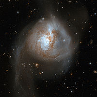
HST image of NGC3256 (credit: NASA, ESA, the Hubble Heritage Team (STScI/AURA)-ESA/Hubble Collaboration and A. Evans (University of Virginia, Charlottesville/NRAO/Stony Brook University)
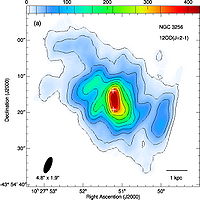
SMA map of CO (2–1) emission in the center of NGC 3256 (Sakamoto, Ho & Peck, 2006)
The luminous infrared galaxy NGC 3256 is the brightest galaxy within ~40 Mpc. This galaxy, which is in the later stages of a merger between two gas-rich progenitors, hosts an extreme central starburst that can be seen across a wide range of wavelengths but emits most strongly in the far infrared (Smith & Harvey 1996). Hubble Space Telescope optical imaging has revealed hundreds of bright young clusters in the galactic center (Trancho et al. 2007). There is also strong evidence for a superwind in NGC 3256, indicating strong starburst-driven blow-out of the interstellar medium (Heckman et al. 2000). Imaging in the infrared, radio and X-rays has shown that NGC 3256 has two distinct nuclei aligned in the north-south direction and separated by 5 arcsec, or 850 pc, on the sky. The southern nucleus is highly obscured, rendering it invisible in the optical.
Because of its proximity and the fact that it is observed nearly face-on, NGC 3256 is an ideal target to study merger-induced starbursts in the local Universe. In fact, NGC 3256 could be regarded as the southern sky equivalent of Arp 220, the archetype of infrared-luminous merging galaxies.
Neutral gas in this galaxy was first studied by English et al (2003), who detected two HI tidal tails that extend up to 50 kpc. High-resolution observations of carbon-monoxide (CO 2-1) in NGC 3256 were made by Sakamoto et al. (2006) using the Submillimeter Array (SMA). This study revealed a large disk of molecular gas (r > 3 kpc) in the center of the merger, with a strong gas concentration toward the double nucleus. This gas disk rotates around a point between the two nuclei. In addition, high-velocity molecular gas was discovered at the galaxy's center, with velocities up to 420 km/s offset from the systemic velocity of the galaxy.
ALMA Data Overview
ALMA Science verification data on NGC3256 in Band 3 were taken in six different
datasets over two consecutive nights: April 16-17, 2011. There are three datasets
for April 16th and three for April 17th. These Band 3 observations utilized all four
available basebands, which are associated with four different spectral windows: two
in the Upper Sideband (USB) and two in the Lower Sideband (LSB). The first spectral
window is centered on the CO(1-0) emission line in the galaxy NGC 3256 and is our
highest frequency spectral window. There is one additional spectral window in the
Upper Side Band (USB), and there are two spectral windows in the Lower Side Band
(LSB). These additional spectral windows are used to measure the continuum emission
in the galaxy and may contain other emission lines as well. Each spectral window
has a total bandwidth of 2 GHz divided over 128 channels, for a channel width of
15.625 MHz, corresponding to about 40 km/s. Online Hanning smoothing was applied to
the data, resulting in a spectral resolution that is twice the channel separation.
For the antenna configuration that was used during these observations, the angular
resolution is expected to be about 6.5".
Due to unfortunate weather conditions during the days planned for these
observations, the data were taken at Band 3 although no previous interferometric
CO(1-0) observations of this galaxy exist. Casoli et al. (1990) observed the CO(1-0)
line with the SEST 15 single dish telescope and were just able to measure a velocity
field with 22" resolution. Interferometric observations were first made with the SMA
in the CO(2-1) line by Sakamoto, Ho & Peck (2006). Because those observations were
made at a higher frequency, the angular resolution is higher (~2") than that of the
ALMA observations shown here, taken in a very compact configuration. Nonetheless, it
is possible to make a direct comparison of the distribution and velocity of the
CO(2-1) and (1-0) gas by looking, for example, at the south-western clump and the
north-eastern 'arm', which are consistent in both data sets.
We thank the following people for suggesting NGC3256 for ALMA Science Verification:
Kazushi Sakamoto, Satoki Matsushita.
Obtaining the Data
To download the data, click on the region closest to your location:
North America
Europe
East Asia
Here you will find three gzipped tar files which, after unpacking, will create three directories:
- NGC3256_Band3_UnCalibratedMSandTablesForReduction - Here we provide you with "starter" datasets, where we have taken the raw data in ALMA Science Data Model (ASDM) format and converted them to CASA Measurement Sets (MS). We did this using the importasdm task in CASA. Along with the raw data, we also provide some tables that you will need for the calibration which cannot currently be generated inside of CASA (for Early Science, these tables will either be pre-applied or supplied with the data).
- NGC3256_Band3_CalibratedData - The fully-calibrated uvdata, ready for imaging and self-calibration
- NGC3256_Band3_ReferenceImages - The final continuum and spectral line images
To see which files you will need, read on below. The downloads to your local computer will take some time, so you may wish to begin them now.
NOTE: CASA 3.3 or later is required to follow this guide. For more information on obtaining the latest version of CASA, see http://casa.nrao.edu.
NGC3256 Data Reduction Tutorial
In this tutorial, or "casaguide", we will guide you step-by-step through the reduction of the ALMA science verification data on NGC3256 and its subsequent imaging. This casaguide consists of two parts:
1) NGC3256 Band3 - Calibration
2) NGC3256 Band3 - Imaging
To complete the Calibration section of the tutorial, you will need the data in the first directory: NGC3256_Band3_UnCalibratedMSandTablesForReduction. For those wishing to skip the calibration section and proceed to Imaging, we also provide the fully-calibrated data in the NGC3256_Band3_CalibratedData directory. Finally, we provide the final continuum and spectral line images in the NGC3256_Band3_ReferenceImages directory.
For a similar tutorial on the reduction of ALMA Band 7 data on TW Hydra, see the casaguide TWHydraBand7.
How to use this casaguide
For both portions of the guide, we will provide you with the full CASA commands needed to carry out each step.
# In CASA
The commands you need to execute
will be displayed in regions
like this.
Simply copy and paste the commands in order into your CASA terminal. You may also type the commands in by hand if desired, but be mindful of typos. Note that you may need to hit Enter twice in order for the process to start running. Also note that copying and pasting multiple commands at a time may not work, so only copy and paste the contents of one region at a time.
To learn how to extract the CASA commands into an executable python script, click here.
Occasionally we will also show output to the CASA logger:
This output will be displayed
in regions like this.
For a brief introduction to the different ways CASA can be run, see the EVLA_Spectral_Line_Calibration_IRC+10216#How_to_Use_This_casaguide page. For further help getting started with CASA, see Getting_Started_in_CASA.
Martin Zwaan, Jacqueline Hodge 07:18 UT, 31 May 2011
Last checked on CASA Version 3.3.0.

