MRK 6: red-shifted HI absorption 5.5.0: Difference between revisions
| Line 46: | Line 46: | ||
{| border=1 | {| border=1 | ||
| '''Source''' || | | '''Source''' || MKN6 | ||
|- | |- | ||
| '''Amp Cal''' || 1328+307 = 3C286 | | '''Amp Cal''' || 1328+307 = 3C286 | ||
| Line 58: | Line 58: | ||
<source lang="python"> | <source lang="python"> | ||
sourceName = " | sourceName = "MKN6" | ||
phaseCal = "1003+830" | phaseCal = "1003+830" | ||
ampCal = "1328+307" | ampCal = "1328+307" | ||
Revision as of 15:28, 4 February 2010
Overview
This example demonstrates a trickier spectral line data set. In this case, several radio bright active galaxies were observed to look for redshifted 21 cm absorption. The data were obtained using 4IF mode, which means that the full range of velocities were split into two spectral windows. Producing the data cube will require eventually stitching these windows back together.
Download your data from the VLA Archive; in this example we'll use the publicly available survey AB658. These data were published in Gallimore et al. (1999).
With the present archive defaults, you should have obtained the following VLA archive files.
'AB658_A921122.xp1'
'AB658_A921122.xp2'
'AB658_A921122.xp3'
'AB658_A921122.xp4'
This tutorial broadly follows the techniques described in the continuum survey tutorial and the 21 cm emission tutorial, and the basic calibration steps are presented only in outline.
Loading the Data
Recall that the python file globber glob is your friend here!
measurementSet = "ab658.ms" # Store the desired name of the measurement set

from glob import glob
fileList = sorted(glob("AB658*.xp?"))

# double check to see if the file already exists
import os

if not os.path.isdir("./" + measurementSet): # measurement sets are directories
    importvla(archivefiles=fileList, vis=measurementSet) # only import if ab658.ms doesn't yet exist

vis = measurementSet
mode = "summary"
vishead
For the purposes of this tutorial, we are interested only in the source Markarian 6, but the reduction techniques could be applied to any of the sources in the measurement set.
Using listobs and plotxy we learn the source names and viable reference antennas.
| Source | MKN6 |
| Amp Cal | 1328+307 = 3C286 |
| Phase Cal | 1003+830 |
| Central Antennas | VA27, VA09, VA23 |
It's just as well to put that information into python global variables.
sourceName = "MKN6"
phaseCal = "1003+830"
ampCal = "1328+307"
refAnt = "VA27" # or perhaps "VA09" or "VA23"
Editing the Data

First inspect the data using plotms.
default(plotms)
vis = measurementSet
field = ampCal
plotms
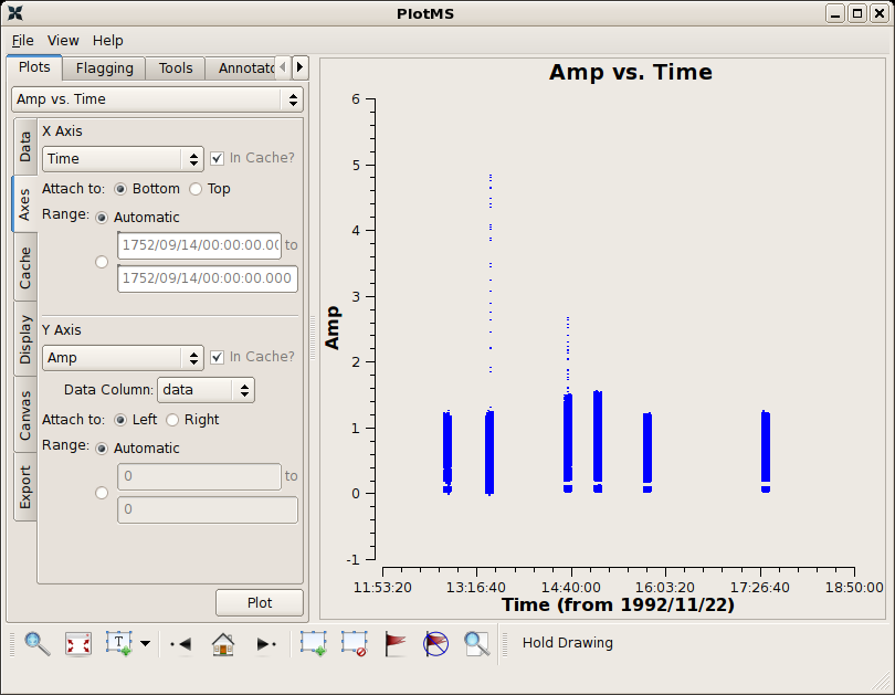
Be sure to select Axes → X Axis → Time and Axes → Y Axis → Amp (those settings are likely the default). There is some obvious junk isolated in time; see the screenshot at right. Follow the tutorial to flag discrepant data for this, the amplitude calibrator, as well as the source and phase calibrator.