M100 Band3 Combine 5.4
Overview
This guide describes how to combine the 7m and 12m interferometric data and then how to feather the resulting image with the total power TP image. All of the data for this Science Verification (SV) project can be found at https://almascience.nrao.edu/alma-data/science-verification. This guide has been written for data reduced in CASA 5.4.0 and assumes that all calibration tables (Tsys and gain tables) have been applied to the visibility weights using calwt=True. If either of these is not the case for your data, do not follow this guide, instead look at https://casaguides.nrao.edu/index.php/DataWeightsAndCombination for methods to correct the data weights for data reduced in earlier versions of CASA.
In order to run this guide you will need the following three files:
- 12m array calibrated data: M100_Band3_12m_CalibratedData.ms
- 7m array calibrated data: M100_Band3_7m_CalibratedData.ms
- Total Power image: M100_TP_CO_cube.spw3.image.bl
To obtain the fully calibrated 12m data M100_Band3_12m_CalibratedData.ms, either download the file M100_Band3_12m_CalibratedData.tgz or download the uncalibrated 12m data (M100_Band3_12m_UnalibratedData.tgz) and execute the calibration scripts (M100_Band3_12m_CalibrationScripts.tgz). How to obtain the data is described in M100_Band3#Obtaining the Data. An overview of the 12m data and its calibration is located at M100_Band3.
WARNING: Note that the imaging presented in this Guide uses the new calibration (using CASA 4.3)
of the same 12-m array data that were released previously (using CASA 3.3).

Do not use the previously released CASA 3.3 version of the calibrated 12-m data (either downloaded
before 28 July 2015 or identified by the suffix "_CASA3.3" after 28 July 2015) for this tutorial.
To obtain the fully calibrated 7m data M100_Band3_7m_CalibratedData.ms, either download the file M100_Band3_7m_CalibratedData.tgz or download the uncalibrated 7m data (M100_Band3_7m_UnalibratedData.tgz) and execute the calibration scripts (M100_Band3_7m_CalibrationScripts.tgz). How to obtain the data is described in M100_Band3#Obtaining the Data. An overview of the 7m data and its calibration is located at M100_Band3.
To obtain the Total Power image M100_TP_CO_cube.spw3.image.bl, either run the M100_Band3_SingleDish guide to calibrate and image the Total Power data or download the image file from M100_Band3_ACA_ReferenceImages.tgz. How to obtain the data is described in M100_Band3#Obtaining the Data. An overview of the Total Power data and its calibration is located at M100_Band3.
Confirm your version of CASA
This guide has been written for CASA release 5.4.0. Please confirm your version before proceeding.
# In CASA
import casadef
version = casadef.casa_version
print "You are using " + version
if (version < '5.1.1'):
    print "YOUR VERSION OF CASA IS TOO OLD FOR THIS GUIDE."
    print "PLEASE UPDATE IT BEFORE PROCEEDING."
else:
    print "Your version of CASA is appropriate for this guide."
Combine and Image the 7m+12m Interferometric Data
Split off CO spectral windows (SPWs)
Use the split and concat commands in M100_Band3_7m_Imaging.py and M100_Band3_12m_Imaging.py available from M100_Band3#Obtaining the Data to create the measurement sets to image in this section.
# In CASA
os.system('rm -rf M100_*m.ms.listobs')
listobs('M100_Band3_12m_CalibratedData.ms',listfile='M100_12m.ms.listobs')
listobs('M100_Band3_7m_CalibratedData.ms',listfile='M100_7m.ms.listobs')
Running the task "listobs" provides the setups used in the observations at a glance. Below are the first target scans of the 12m and 7m observations and the spectral window tables as generated by listobs; these are excerpts from the complete files obtained in each case. Notice that the six 7m data sets were taken with two slightly different correlator setups (one with four SPWs and the other with two SPWs), so the concatenated data set has six total SPWs.
12m data:
ObservationID = 0         ArrayID = 0
  Date        Timerange (UTC)          Scan  FldId FieldName             nRows     SpwIds   Average Interval(s)    ScanIntent
  10-Aug-2011/19:38:05.8 - 19:50:22.8    11      1 M100                      1500  [0,1,2,3]  [6.05, 6.05, 6.05, 6.05] [CALIBRATE_WVR#ON_SOURCE,OBSERVE_TARGET#ON_SOURCE]

Spectral Windows:  (4 unique spectral windows and 1 unique polarization setups)
  SpwID  Name   #Chans   Frame   Ch0(MHz)  ChanWid(kHz)  TotBW(kHz) CtrFreq(MHz) BBC Num  Corrs
  0              3840   TOPO  113726.419       488.281   1875000.0 114663.6750        1  XX  YY
  1              3840   TOPO  111851.419       488.281   1875000.0 112788.6750        2  XX  YY
  2              3840   TOPO  103663.431      -488.281   1875000.0 102726.1750        3  XX  YY
  3              3840   TOPO  101850.931      -488.281   1875000.0 100913.6750        4  XX  YY
7m data:
ObservationID = 0         ArrayID = 0
  Date        Timerange (UTC)          Scan  FldId FieldName             nRows     SpwIds   Average Interval(s)    ScanIntent
  17-Mar-2013/04:44:04.3 - 04:50:43.7    11      1 M100                       261  [0,1,2,3]  [10.1, 10.1, 10.1, 10.1] [OBSERVE_TARGET#ON_SOURCE]

Spectral Windows:  (6 unique spectral windows and 1 unique polarization setups)
  SpwID  Name                           #Chans   Frame   Ch0(MHz)  ChanWid(kHz)  TotBW(kHz) CtrFreq(MHz) BBC Num  Corrs
  0      ALMA_RB_03#BB_1#SW-01#FULL_RES   4080   TOPO  101945.850      -488.281   1992187.5 100950.0000        1  XX  YY
  1      ALMA_RB_03#BB_2#SW-01#FULL_RES   4080   TOPO  103761.000      -488.281   1992187.5 102765.1500        2  XX  YY
  2      ALMA_RB_03#BB_3#SW-01#FULL_RES   4080   TOPO  111811.300       488.281   1992187.5 112807.1500        3  XX  YY
  3      ALMA_RB_03#BB_4#SW-01#FULL_RES   4080   TOPO  113686.300       488.281   1992187.5 114682.1500        4  XX  YY
  4      ALMA_RB_03#BB_1#SW-01#FULL_RES   4080   TOPO  111798.250       488.281   1992187.5 112794.1000        1  XX  YY
  5      ALMA_RB_03#BB_2#SW-01#FULL_RES   4080   TOPO  113673.250       488.281   1992187.5 114669.1000        2  XX  YY


Examination of the listobs files shows that the CO is in SPW='0' for the 12m data and in SPW='3,5' for the 7m data. There are two SPWs containing CO in the 7m data due to the slightly differing correlator setups.
Also note that the integration time per visibility (average interval parameter in listobs) is different: 6.05s for the 12m data and 10.1s for the 7m. This will be important to know later when we check the visibility weights.
Next we split out the CO spectral windows.
# In CASA
os.system('rm -rf M100_12m_CO.ms')
split(vis='M100_Band3_12m_CalibratedData.ms',
      outputvis='M100_12m_CO.ms',spw='0',field='M100',
      datacolumn='data',keepflags=False)
os.system('rm -rf M100_7m_CO.ms')
split(vis='M100_Band3_7m_CalibratedData.ms',
      outputvis='M100_7m_CO.ms',spw='3,5',field='M100',
      datacolumn='data',keepflags=False)
Also of interest is that the 12m data has 47 fields and the 7m has 23 fields (not shown in the listobs excerpts above). The difference in number of pointings is because the 7m antennas have a FWHP (full width half power) primary beam diameter that is 12/7 times larger than the 12m antennas. One easy way to see how the mosaics compare is to install the AnalysisUtils package (see Analysis_Utilities for information on how to download and import AnalysisUtils). Then with AnalysisUtils you can make the following plots (look at the listobs to obtain the sourceid):
# In CASA
os.system('rm -rf *m_mosaic.png')
au.plotmosaic('M100_12m_CO.ms',sourceid='0',doplot=True,figfile='12m_mosaic.png')
au.plotmosaic('M100_7m_CO.ms',sourceid='0',doplot=True,figfile='7m_mosaic.png')
We see that the mosaics cover a common area but that the 7m mosaic is a bit larger. This means that the outer edges of the combined mosaic will be noisier than expected if they overlapped perfectly; this is just something to keep in mind. If you had the case where the mosaic coverages are dramatically different, it would be best to exclude the completely non-overlapping fields from the combination.
NOTE: At this stage one would typically do continuum subtraction (if there is any). However we already know from the individual data reductions that the 3mm continuum emission is quite weak and does not significantly contribute to a 5km/s channel, so we will forgo the the continuum subtraction step. Examples of how to do this if you are so inclined are located in various other ALMA CASAguides.
Checking the weights and concatenating the data
When combining data with disparate properties it is very important that the relative weights of each visibility be in the correct proportion to the other data according to the radiometer equation. Formally, the visibility weights should be proportional to 1/sigma2 where sigma is the variance or rms noise of a given visibility.
The rms noise in a single channel for a single visibility is:
[math]\displaystyle{ \sigma_{ij} (Jy) =\frac{2k}{\eta_{q}\eta_{c}A_{eff}} }[/math] [math]\displaystyle{ \sqrt{\frac{T_{sys,i} T_{sys,j}}{2\Delta\nu_{ch} t_{ij}}} }[/math] [math]\displaystyle{ \times 10^{26}, }[/math]
where:
k is Boltzmann's constant.
Aeff is the effective antenna area which is equal to the aperture efficiency x the geometric area of the antenna. The aperture efficiency depends on the rms antenna surface accuracy.
ηq and ηc are the quantization and correlator efficiencies, respectively. These have values near 1 and will be ignored for the purposes of this casaguide, but see the ALMA Technical Handbook for more information.
Tsys,i is the system temperature for antenna i, and Tsys,j is the system temperature for antenna j
Δνch is the channel frequency width.
tij is the integration time per visibility.

In CASA versions > 4.3.1, the weights are intially scaled by 2ΔνchΔtij, and after the Tsys table applycal step of the calibration process, further scaled by 1/[(Tsys(i) * Tsys(j)] as long as calwt=True. In the subsequent amplitude gain calibration table applycal step of the calibration, the weights are further scaled by a factor of [gain(i)2 * gain(j)2] if calwt=True. This step up-weights data from the best performing antennas from the gain point of view, and importantly for data combination, makes the weights correctly proportional to the antenna size.

In the calibration scripts for all executions of the 12m and 7m data, both applycal steps set calwt=True. To verify that the weights come out as expected, we plot the weights of the 7m and 12m data and measure their ratio to be, on average, 7m/12m ~ 0.055/0.3 ~ 0.18. Note that in the plots the points are colored by SPW, so there is only one 12m CO SPW but there are two 7m CO SPWs, and that no averaging can be turned on when plotting the weights.
# In CASA
os.system('rm -rf 7m_WT.png 12m_WT.png')
plotms(vis='M100_12m_CO.ms',yaxis='wt',xaxis='uvdist',spw='0:200',
       coloraxis='spw',plotfile='12m_WT.png',showgui=True)
#
plotms(vis='M100_7m_CO.ms',yaxis='wt',xaxis='uvdist',spw='0~1:200',
       coloraxis='spw',plotfile='7m_WT.png',showgui=True)
The two key things that are different between the 7m and 12m-array data are that the effective dish areas are different by (7/12)2, and the integration times are different by (10.1/6.05). Since the dish area and the integration time per visibility are in the denominator of the radiometer equation, and assuming the weight of an individual visibility is proportional to 1/sigma2, the ratio of the weights should be (7./12.)4 x (10.1/6.05) = 0.19. This is very close to the value we measure for the ratio of the weights, particularly given that the 7m flux calibration relied on a source which changed substantially over the course of the six 7m-array observations. Recent ALMA calibrations (CASA > 4.3.1) should have all of these details correctly accounted for; older calibrated data may not, in which case the reader should consult https://casaguides.nrao.edu/index.php/DataWeightsAndCombination (or simply recalibrate the data in the latest release using calwt=True).
Now concatenate the two data sets and plot the concatenated weights to verify that they are as expected.

# In CASA
# Concate; scale weights using visweightscale if applicable (old calibrations)
os.system('rm -rf M100_combine_CO.ms')
concat(vis=['M100_12m_CO.ms','M100_7m_CO.ms'],
       concatvis='M100_combine_CO.ms')

# In CASA
os.system('rm -rf combine_CO_WT.png')
plotms(vis='M100_combine_CO.ms',yaxis='wt',xaxis='uvdist',spw='0~2:200',
       coloraxis='spw',plotfile='combine_CO_WT.png',showgui=True)
Here, we create more instructive plots of the combined data to check that things are in order. (Let each plot finish before cutting and pasting next plot. If plotms gui disappears, exit CASA and restart.)
One way to assess the relative noise in the combined data is to plot amplitude as a function of uv-distance. Here, it's clear that the 7m data is noisier than the 12m data (note also that this plot is not shown):
# In CASA
os.system('rm -rf M100_combine_uvdist.png')
plotms(vis='M100_combine_CO.ms',yaxis='amp',xaxis='uvdist',spw='', avgscan=True,
       avgchannel='5000', coloraxis='spw',plotfile='M100_combine_uvdist.png',showgui=True)
A fairer comparison of these data is achieved by isolating the brightest line channels in individual 12m and 7m data sets (i.e., not the concatenated data sets) and comparing only those channels in amplitude vs. uv-distance. Here the agreement is better, as it is less dominated by the scatter among the several 7m executions.

To plot the CO line as a function of velocity (this plot takes a while):
# In CASA
os.system('rm -rf M100_combine_vel.png')
plotms(vis='M100_combine_CO.ms',yaxis='amp',xaxis='velocity',spw='', avgtime='1e8',avgscan=True,coloraxis='spw',avgchannel='5',
       transform=True,freqframe='LSRK',restfreq='115.271201800GHz', plotfile='M100_combine_vel.png',showgui=True)
To see each spectral window independently in plotms, run the command again but remove the call to "plotfile" and add " iteraxis='spw' ".
Joint (7m+12m) Image Deconvolution using TCLEAN
The commands below use the built in auto-masking available in tclean. For more information, see Automasking_Guide.
Note that even if these data had only been comprised of a single pointing of 7m and 12m-array data, the gridder='mosaic' mode would be needed to correctly image data with different antenna sizes.
The commands have been split into multiple sections to aid cut and paste. Wait until the current one is done before starting the next section. If you stop CASA and restart you will need to cut and paste again from the Define Parameters section on down.
Any time it is necessary to enter a long series of commands, typing %cpaste before the start of the series and -- at the end of the series lets CASA know that there are more commands coming. This can be very helpful when needing to cut and paste a lot of lines at once. In particular, indentations in the code (like loops in the example below) may not be parsed correctly in a straight cut-and-paste. These commands are not explicitly included in any of the sets of commands below, but they can be applicable for any of them.
Define Parameters
Note that the parameters used here--- other than the gridder parameter, as noted above--- are by design the same as those used to make the stand-alone 7m-array and 12m-array images.
# In CASA

### Define clean parameters
vis='M100_combine_CO.ms'
prename='M100_combine_CO_cube'
imsize=800
cell='0.5arcsec'
minpb=0.2
restfreq='115.271201800GHz'
outframe='LSRK'
spw='0~2'
width='5km/s'
start='1400km/s'
nchan=70
robust=0.5
phasecenter='J2000 12h22m54.9 +15d49m15'

### Setup stopping criteria with multiplier for rms.
stop=3.
Make Initial Dirty Image and Determine Synthesized Beam area
The dirty image is used to determine the rms and threshold for cleaning.
# In CASA
### Make initial dirty image
os.system('rm -rf '+prename+'_dirty.*')
tclean(vis=vis,
    imagename=prename + '_dirty',
    gridder='mosaic',
    deconvolver='hogbom',
    pbmask=minpb,
    imsize=imsize,
    cell=cell,
    spw=spw,
    weighting='briggs',
    robust=robust,
    phasecenter=phasecenter,
    specmode='cube',
    width=width,
    start=start,
    nchan=nchan,
    restfreq=restfreq,
    outframe=outframe,
    veltype='radio',
    restoringbeam='common',
    mask='',
    niter=0,
    interactive=False)
Find properties of the dirty image
# In CASA
### Find the peak in the dirty cube.
myimage=prename+'_dirty.image'
bigstat=imstat(imagename=myimage)
peak= bigstat['max'][0]
print 'peak (Jy/beam) in cube = '+str(peak)

# find the RMS of a line free channel (should be around 0.011
chanstat=imstat(imagename=myimage,chans='4')
rms1= chanstat['rms'][0]
chanstat=imstat(imagename=myimage,chans='66')
rms2= chanstat['rms'][0]
rms=0.5*(rms1+rms2)

print 'rms (Jy/beam) in a channel = '+str(rms)
Clean the Data
We will use the auto-masking option in tclean to non-interactively clean the data. The thresholds used come from the suggested values found in the Automasking_Guide. The threshold is set to 3 times the dirty cube RMS. Note: Auto-masking has not been extensively tested using the deconvolver='multiscale'. If you are using your own data, you may need to modify the threshold parameters and/or use multiscale clean.
In CASA version 5.4 there is a new parameter that is necessary, mosweight=True. This is a subparameter of the mosaic gridder which determines whether to weight each field in a mosaic independently (if True) or to calculate the weight density from the average uv distribution of all the fields combined (if False). You should also take care in choosing the Briggs Robust weighting value. For mosaics, robust values less than 0 are not recommended. For more information about weighting see tclean.
# In CASA

sidelobethresh = 2.0
noisethresh = 4.25
minbeamfrac = 0.3
lownoisethresh= 1.5
negativethresh = 0.0

os.system('rm -rf ' + prename + '.*')
tclean(vis=vis,
    imagename=prename,
    gridder='mosaic',
    deconvolver='hogbom',
    pbmask=minpb,
    imsize=imsize,
    cell=cell,
    spw=spw,
    weighting='briggs',
    robust=robust,
    phasecenter=phasecenter,
    specmode='cube',
    width=width,
    start=start,
    nchan=nchan,
    restfreq=restfreq,
    outframe=outframe,
    veltype='radio',
    restoringbeam='common',
    mosweight=True,
    niter=10000,
    usemask='auto-multithresh',
    threshold=str(stop*rms)+'Jy/beam',
    sidelobethreshold=sidelobethresh,
    noisethreshold=noisethresh,
    lownoisethreshold=lownoisethresh,
    minbeamfrac=minbeamfrac,
    growiterations=75,
    negativethreshold=negativethresh,
    interactive=False,
    pbcor=True)
Image Analysis for the 7m+12m Data
Moment Maps for 7m+12m CO (1-0) Cube
Start by examining the final image cube. Determine the start and stopping channels for the line emission -- this will be used in the "chans" parameter of immoments.
# In CASA
viewer('M100_combine_CO_cube.image',gui=True)
Next determine the rms noise per channel and use that to exclude pixels from the moment images. All images are shown in the gallery at the end of the following section.
# In CASA
myimage='M100_combine_CO_cube.image'
chanstat=imstat(imagename=myimage,chans='4')
rms1= chanstat['rms'][0]
chanstat=imstat(imagename=myimage,chans='66')
rms2= chanstat['rms'][0]
rms=0.5*(rms1+rms2)
print 'rms in a channel = '+str(rms)
Next make the moment maps. For the integrated intensity: moment 0, a 2 sigma cut often considerably improves the appearance of the image with little effect on the integrated intensity as long as emission free channels are excluded. For higher order moments it is necessary to exclude all low S/N data. Typically 5-6 sigma for the higher moments works well. We also apply further masking based on the .pb image because the edges of the combined mosaic are especially noisy because the 7m mosaic is somewhat larger than the 12m mosaic as described above (see Figures 1 & 2).
# In CASA
os.system('rm -rf M100_combine_CO_cube.image.mom0')
immoments(imagename = 'M100_combine_CO_cube.image',
         moments = [0],
         axis = 'spectral',chans = '9~61',
         mask='M100_combine_CO_cube.pb>0.3',
         includepix = [rms*2,100.],
         outfile = 'M100_combine_CO_cube.image.mom0')

os.system('rm -rf M100_combine_CO_cube.image.mom1')
immoments(imagename = 'M100_combine_CO_cube.image',
         moments = [1],
         axis = 'spectral',chans = '9~61',
         mask='M100_combine_CO_cube.pb>0.3',
         includepix = [rms*5.5,100.],
         outfile = 'M100_combine_CO_cube.image.mom1')
Now we can make some figures showing the moment maps.
# In CASA
os.system('rm -rf M100_combine_CO_cube.image.mom*.png')
imview (raster=[{'file': 'M100_combine_CO_cube.image.mom0',
                 'range': [-0.3,25.],'scaling': -1.3,'colorwedge': True}],
         zoom={'blc': [190,150],'trc': [650,610]},
         out='M100_combine_CO_cube.image.mom0.png')

imview (raster=[{'file': 'M100_combine_CO_cube.image.mom1',
                 'range': [1440,1695],'colorwedge': True}],
         zoom={'blc': [190,150],'trc': [650,610]},
         out='M100_combine_CO_cube.image.mom1.png')
If you plan to use your moment 0 image to make measurements, it needs to be primary beam corrected first. First we need to subimage the .pb cube to extract a single plane that can be used to primary beam correct the moment 0 image.
# In CASA
os.system('rm -rf M100_combine_CO_cube.pb.1ch')
imsubimage(imagename='M100_combine_CO_cube.pb',
           outfile='M100_combine_CO_cube.pb.1ch',
           chans='35')
Next, primary beam correct the moment 0 image. This is the version that would be used for measurements, though the uncorrected one can be useful for figures. The difference is clear in the images seen below in the following section.
# In CASA
os.system('rm -rf M100_combine_CO_cube.image.mom0.pbcor')
impbcor(imagename='M100_combine_CO_cube.image.mom0',
    pbimage='M100_combine_CO_cube.pb.1ch',
    outfile='M100_combine_CO_cube.image.mom0.pbcor')
Have a look at the difference the primary beam correction makes.
# In CASA
imview (raster=[{'file': 'M100_combine_CO_cube.image.mom0',
                 'range': [-0.3,25.],'scaling': -1.3},
                {'file': 'M100_combine_CO_cube.image.mom0.pbcor',
                 'range': [-0.3,25.],'scaling': -1.3}],
         zoom={'blc': [190,150],'trc': [650,610]})
With the viewer open, you can flip back and forth between the images to compare them. Next, make a figure.
# In CASA
os.system('rm -rf M100_combine_CO_cube.image.mom0.pbcor.png')
imview (raster=[{'file': 'M100_combine_CO_cube.image.mom0.pbcor',
                 'range': [-0.3,25.],'scaling': -1.3,'colorwedge': True}],
         zoom={'blc': [190,150],'trc': [650,610]},
         out='M100_combine_CO_cube.image.mom0.pbcor.png')
Comparison with 7m, 12m Moment Maps
Below the moment maps from the 7m-only and the 12m-only data are shown for comparison. The moment maps were made using clean masks drawn by hand for comparison to the automasking technique; the two appear to be qualitatively similar. Details on the creation of these images (masking, thresholding, and the number of iterations of clean) can be found within the 12m and 7m imaging scripts available with the downloaded package. The range and scaling for the 12m-only figures are the same as that used for the 7m+12m figures for ease of comparison.
As expected, the 7m+12m image shows considerably more extended emission than the 12m-only data and finer detail than the 7m-only data. For comparison, the 7m+12m synthesized beam is 3.80"x2.50", while the 12m-only beam is 3.46"x2.37" and the 7m-only beam is 12.72"x10.12".
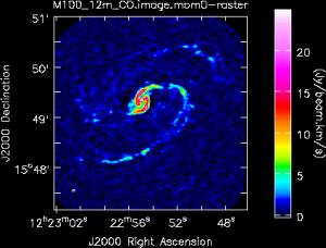
Moment 0 for 12m data alone (no primary beam correction).
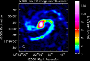
Moment 0 for 7m data alone (no primary beam correction).
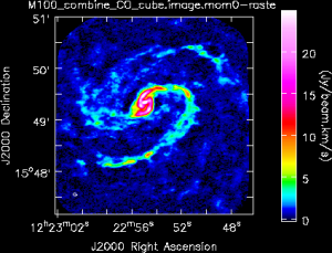
Moment 0 for 12m+7m data (no primary beam correction).
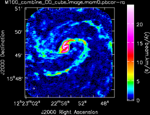
Moment 0 for 12m+7m data with primary beam correction.


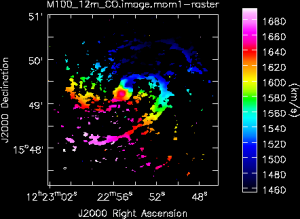
Moment 1 for 12m data alone.
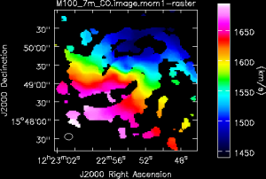
Moment 1 for 7m data alone.
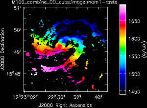
Moment 1 for 12m+7m data.


Convert 7m+12m Images to Fits Format
# In CASA
os.system('rm -rf *.fits')
exportfits(imagename='M100_combine_CO_cube.image',fitsimage='M100_combine_CO_cube.image.fits')

exportfits(imagename='M100_combine_CO_cube.pb',fitsimage='M100_combine_CO_cube.pb.fits')

exportfits(imagename='M100_combine_CO_cube.image.mom0',fitsimage='M100_combine_CO_cube.image.mom0.fits')

exportfits(imagename='M100_combine_CO_cube.image.mom0.pbcor',fitsimage='M100_combine_CO_cube.image.mom0.pbcor.fits')

exportfits(imagename='M100_combine_CO_cube.image.mom1',fitsimage='M100_combine_CO_cube.image.mom1.fits')
Feathering the Total Power and 7m+12m Interferometric Images
In this section the interferometric (7m+12m) image produced above is combined with the Total Power (single dish) image. The "feather" algorithm is employed, in which the two images are combined in the spatial frequency domain, i.e., the low and high spatial frequency components are predominantly taken from the TP and interferometric images, respectively.
Prepare Images for Feathering
When feathering, it is important to ensure that the rest frequency used in the creation of the single-dish and array cubes was the same. For pipeline-produced TP cubes, this may not be the case. You can check the rest frequencies for the cubes in CASA using imhead:
#In CASA
imhead('M100_TP_CO_cube.spw3.image.bl',mode='get',hdkey='restfreq')
imhead('M100_combine_CO_cube.image',mode='get',hdkey='restfreq')
In this case, the rest frequencies match and we can go ahead with the regridding and feathering steps. If the values differ, however, you can use the casa task imreframe to change the rest frequency, and consequently, the velocity axis, of your total power cube to match your interferometric data.
Regrid the TP image to match the shape of the 7m+12m image using the task imregrid. The TP image is resampled onto the same grid as that of the "template" 7m+12m image along the first two axes of the cube (i.e., RA and Dec; it is not necessary to regrid the velocity axis, since the axis is already common to the both images).
#In CASA
os.system('rm -rf M100_TP_CO_cube.regrid')
imregrid(imagename='M100_TP_CO_cube.spw3.image.bl',
         template='M100_combine_CO_cube.image',
         axes=[0, 1],
         output='M100_TP_CO_cube.regrid')
Now we trim the 7m+12m and (regridded) TP images, in order to exclude the regions masked by the clean task with minpb=0.2 and/or noisy edge regions in the TP image. The viewer task can be used to determine the trimming box. Here we use (x, y) = (219, 148) and (612, 579) [pixels] as the bottom-left and top-right corners, respectively, and set these values to the "box" parameter of the imsubimage task.
#In CASA
os.system('rm -rf M100_TP_CO_cube.regrid.subim')
imsubimage(imagename='M100_TP_CO_cube.regrid',
           outfile='M100_TP_CO_cube.regrid.subim',
           box='219,148,612,579')
os.system('rm -rf M100_combine_CO_cube.image.subim')
imsubimage(imagename='M100_combine_CO_cube.image',
           outfile='M100_combine_CO_cube.image.subim',
           box='219,148,612,579')
While the 7m+12m image (before the primary-beam correction) has non-uniform primary beam response (i.e., lower response in the outskirts of the mosaic field), the TP image does not have such non-uniformity. In order to feather the TP and 7m+12m images together, they should have the common response on the sky. Hence we need to multiply the TP image by the 7m+12m primary beam response before proceeding. To do this, create the subimage of the 7m+12m response,
#In CASA
os.system('rm -rf M100_combine_CO_cube.pb.subim')
imsubimage(imagename='M100_combine_CO_cube.pb',
           outfile='M100_combine_CO_cube.pb.subim',
           box='219,148,612,579')
then multiply it and the TP image using the task immath.
#In CASA
os.system('rm -rf M100_TP_CO_cube.regrid.subim.depb')
immath(imagename=['M100_TP_CO_cube.regrid.subim',
                  'M100_combine_CO_cube.pb.subim'],
       expr='IM0*IM1',
       outfile='M100_TP_CO_cube.regrid.subim.depb')
Again, note the warning regarding the different units of the input images in immath.
As a result, the feathered image will have the same response as that of the 7m+12m image. The primary-beam correction can be done after the feathering process (see below).
Feather TP Cube with 7m+12m Cube
Now we are ready to execute the feather task to combine the TP and 7m+12m images.
#In CASA
os.system('rm -rf M100_Feather_CO.image')
feather(imagename='M100_Feather_CO.image',
        highres='M100_combine_CO_cube.image.subim',
        lowres='M100_TP_CO_cube.regrid.subim.depb')
The task produces the combined image in the following way:
- Convert the input images specified by the "highres" and "lowres" parameters onto the spatial frequency plane.
- Combine them on the spatial frequency plane. The weighting is determined by the beam sizes/shapes of the input images.
- Convert it back to the image plane.
Please refer to the online help and documents for the details.
Make Moment Maps of the Feathered Images
We will use the same technique as the 7m+12m image analysis above to make moment maps.
First (but optionally; this is solely for comparison to the feathered images and not needed to create the final feathered images), make moment maps for the (regridded) TP image.
#In CASA
myimage = 'M100_TP_CO_cube.regrid.subim'
chanstat = imstat(imagename=myimage,chans='4')
rms1 = chanstat['rms'][0]
chanstat = imstat(imagename=myimage,chans='66')
rms2 = chanstat['rms'][0]
rms = 0.5*(rms1+rms2)

os.system('rm -rf M100_TP_CO_cube.regrid.subim.mom0')
immoments(imagename='M100_TP_CO_cube.regrid.subim',
         moments=[0],
         axis='spectral',
         chans='10~61',
         includepix=[rms*2., 50],
         outfile='M100_TP_CO_cube.regrid.subim.mom0')

os.system('rm -rf M100_TP_CO_cube.regrid.subim.mom1')
immoments(imagename='M100_TP_CO_cube.regrid.subim',
         moments=[1],
         axis='spectral',
         chans='10~61',
         includepix=[rms*5.5, 50],
         outfile='M100_TP_CO_cube.regrid.subim.mom1')

os.system('rm -rf M100_TP_CO_cube.regrid.subim.mom*.png')
imview(raster=[{'file': 'M100_TP_CO_cube.regrid.subim.mom0',
                'range': [0., 1080.],
                'scaling': -1.3,
                'colorwedge': True}],
       out='M100_TP_CO_cube.regrid.subim.mom0.png')

imview(raster=[{'file': 'M100_TP_CO_cube.regrid.subim.mom1',
                'range': [1440, 1695],
                'colorwedge': True}],
       out='M100_TP_CO_cube.regrid.subim.mom1.png')
Then make moment maps for the feathered image.
#In CASA
myimage = 'M100_Feather_CO.image'
chanstat = imstat(imagename=myimage,chans='4')
rms1 = chanstat['rms'][0]
chanstat = imstat(imagename=myimage,chans='66')
rms2 = chanstat['rms'][0]
rms = 0.5*(rms1+rms2)

os.system('rm -rf M100_Feather_CO.image.mom0')
immoments(imagename='M100_Feather_CO.image',
         moments=[0],
         axis='spectral',
         chans='10~61',
         includepix=[rms*2., 50],
         outfile='M100_Feather_CO.image.mom0')

os.system('rm -rf M100_Feather_CO.image.mom1')
immoments(imagename='M100_Feather_CO.image',
         moments=[1],
         axis='spectral',
         chans='10~61',
         includepix=[rms*5.5, 50],
         outfile='M100_Feather_CO.image.mom1')

os.system('rm -rf M100_Feather_CO.image.mom*.png')
imview(raster=[{'file': 'M100_Feather_CO.image.mom0',
                'range': [-0.3, 25.],
                'scaling': -1.3,
                'colorwedge': True}],
       out='M100_Feather_CO.image.mom0.png')

imview(raster=[{'file': 'M100_Feather_CO.image.mom1',
                'range': [1440, 1695],
                'colorwedge': True}],
       out='M100_Feather_CO.image.mom1.png')
Correct the Primary Beam Response
Apply the primary beam response to the feathered image using the task immath,
#In CASA
os.system('rm -rf M100_Feather_CO.image.pbcor')
immath(imagename=['M100_Feather_CO.image',
                  'M100_combine_CO_cube.pb.subim'],
       expr='IM0/IM1',
       outfile='M100_Feather_CO.image.pbcor')
and also to the moment 0 image.
#In CASA
os.system('rm -rf M100_combine_CO_cube.pb.1ch.subim')
imsubimage(imagename='M100_combine_CO_cube.pb.subim',
           outfile='M100_combine_CO_cube.pb.1ch.subim',
           chans='35')

os.system('rm -rf M100_Feather_CO.image.mom0.pbcor')
immath(imagename=['M100_Feather_CO.image.mom0',
                  'M100_combine_CO_cube.pb.1ch.subim'],
        expr='IM0/IM1',
        outfile='M100_Feather_CO.image.mom0.pbcor')
Save the primary-beam corrected moment 0 image to a PNG file.
#In CASA
os.system('rm -rf M100_Feather_CO.image.mom0.pbcor.png')
imview(raster=[{'file': 'M100_Feather_CO.image.mom0.pbcor',
                'range': [-0.3, 25.],
                'scaling': -1.3,
                'colorwedge': True}],
       out='M100_Feather_CO.image.mom0.pbcor.png')
Compare the Various Images
Now we compare all the images:
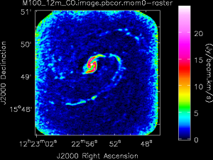
Primary beam corrected moment 0 for the 12m data.
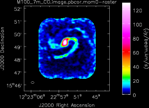
Primary beam corrected moment 0 for the 7m data.
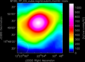
Moment 0 for the TP data.
Primary beam corrected moment 0 for 7m+12m data.
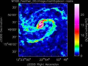
Primary beam corrected moment 0 for TP+7m+12m data.


Moment 1 for 12m data.
Moment 1 for 7m data.
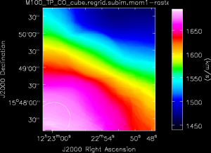
Moment 1 for the TP data.
Moment 1 for 7m+12m data.
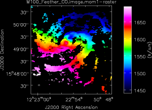
Moment 1 for TP+7m+12m data.


You can see that more extended emission is recovered by adding the TP data to the interferometric data.
For quantitative comparison, we measure the total line fluxes of the various images. The task imstat can be used to do this. For example, for the subimage of the 7m+12m image,
#In CASA
imstat('M100_combine_CO_cube.image.subim')
yields the following:
{'blc': array([0, 0, 0, 0], dtype=int32),
 'blcf': '12:23:01.170, +15.47.08.994, I, 1.14733e+11Hz',
 'flux': array([ 921.95231117]),
 'max': array([ 0.75541693]),
 'maxpos': array([172, 253,   0,  49], dtype=int32),
 'maxposf': '12:22:55.212, +15.49.15.500, I, 1.14639e+11Hz',
 'mean': array([ 0.00084236]),
 'medabsdevmed': array([ 0.00865066]),
 'median': array([-0.00024056]),
 'min': array([-0.09347859]),
 'minpos': array([260, 251,   0,  26], dtype=int32),
 'minposf': '12:22:52.163, +15.49.14.499, I, 1.14683e+11Hz',
 'npts': array([ 11914560.]),
 'q1': array([-0.00888554]),
 'q3': array([ 0.00841561]),
 'quartile': array([ 0.01730115]),
 'rms': array([ 0.02016445]),
 'sigma': array([ 0.02014685]),
 'sum': array([ 10036.30851966]),
 'sumsq': array([ 4844.52212774]),
 'trc': array([393, 431,   0,  69], dtype=int32),
 'trcf': '12:22:47.554, +15.50.44.492, I, 1.146e+11Hz'}
The 'flux' value in the result is the total integrated line flux in Jy km/s, where (in contrast to CASA versions 4.3 or less) the 5 km/s velocity channels are taken into account.
Similarly, the total line fluxes of the TP image (after multiplying the 7m+12m primary beam response), feathered image, and feathered image after the primary-beam correction are
#In CASA
imstat('M100_TP_CO_cube.regrid.subim.depb')['flux']
imstat('M100_Feather_CO.image')['flux']
imstat('M100_Feather_CO.image.pbcor')['flux']
CASA <166>: imstat('M100_TP_CO_cube.regrid.subim.depb')['flux']
Out[166]: array([ 2822.29454956])

CASA <167>: imstat('M100_Feather_CO.image')['flux']
Out[167]: array([ 2822.29259255])

CASA <168>: imstat('M100_Feather_CO.image.pbcor')['flux']
Out[168]: array([ 3055.66039175])
We see the following from these values:
- The flux recovered by the 7m+12m observations is little less than half of the total flux (984/2822 = 0.34).
- The feathering process preserves the flux of the TP data.
- The flux of the primary-beam corrected feathered image is consistent with the values from the literature (2972 +/- 319 Jy km/s from the BIMA SONG; Helfer et al. 2003).
Last checked on CASA Version 5.4.0.