M100 Band3 Combine 4.2.2
Overview
This guide describes how to combine the 7m and 12m interferometric data and then how to feather the resulting image with the total power TP image. All of the data for this SV project can be found at https://almascience.nrao.edu/alma-data/science-verification. In order to run this guide you will need to:
- Either run the 7m casaguide M100_Band3_ACA_4.1 to obtain the final 7m fully calibrated data or download the fully calibrated data: (i.e. M100_Band3_7m_CalibratedData.tgz)
- Either download the new RawUnCalibrated data for the 12m-array and run the new calibration script or download the fully calibrated data (i.e. M100_Band3_12m_CalibratedData.tgz). Note that while these are the same data that were released previously, the data reduction path has been updated to current best practices and starts from the raw data files called ASDMs (ALMA Science Data Model). Do not use the previously released uncalibrated or calibrated data.
- Either run the M100_Band3_SingleDish_4.1 guide to calibrate and image the Total Power data or download the final image (i.e. M100_TP_Image.tgz)
Confirm your version of CASA
This guide has been written for CASA release 4.1.0. Please confirm your version before proceeding.
# In CASA
version = casadef.casa_version
print "You are using " + version
if (version < '4.1.0'):
    print "YOUR VERSION OF CASA IS TOO OLD FOR THIS GUIDE."
    print "PLEASE UPDATE IT BEFORE PROCEEDING."
else:
    print "Your version of CASA is appropriate for this guide."
Combine and Image the 7m+12m Interferometric Data
Split off CO spws
# In CASA
os.system('rm -rf m100_*m.ms.listobs')
listobs('M100_Band3_12m_CalibratedData.ms',listfile='m100_12m.ms.listobs')
listobs('M100_Band3_7m_CalibratedData.ms',listfile='m100_7m.ms.listobs')
Below are the observation and spectral window tables from the listobs.
12m data:

ObservationID = 0         ArrayID = 0
  Date        Timerange (UTC)          Scan  FldId FieldName             nRows     SpwIds   Average Interval(s)
  10-Sep-2011/18:28:43.4 - 18:41:00.4    11      1 M100                      1320  [0, 1, 2, 3]  [6.05, 6.05, 6.05, 6.05]

Spectral Windows:  (4 unique spectral windows and 1 unique polarization setups)
  SpwID  Name   #Chans   Frame   Ch1(MHz)  ChanWid(kHz)  TotBW(kHz) BBC Num  Corrs
  0              3840   TOPO  113726.419       488.281   1875000.0       1  XX  YY
  1              3840   TOPO  111851.419       488.281   1875000.0       2  XX  YY
  2              3840   TOPO  103663.431      -488.281   1875000.0       3  XX  YY
  3              3840   TOPO  101850.931      -488.281   1875000.0       4  XX  YY

7m data:

ObservationID = 0         ArrayID = 0
  Date        Timerange (UTC)          Scan  FldId FieldName             nRows     SpwIds   Average Interval(s)
  17-Mar-2013/04:44:04.3 - 04:50:43.7    11      1 M100                       168  [0, 1]  [10.1, 10.1]

Spectral Windows:  (4 unique spectral windows and 1 unique polarization setups)
  SpwID  Name                           #Chans   Frame   Ch1(MHz)  ChanWid(kHz)  TotBW(kHz) BBC Num  Corrs
  0      ALMA_RB_03#BB_3#SW-01#FULL_RES   4080   TOPO  111811.300       488.281   1992187.5       3  XX  YY
  1      ALMA_RB_03#BB_4#SW-01#FULL_RES   4080   TOPO  113686.300       488.281   1992187.5       4  XX  YY
  2      ALMA_RB_03#BB_1#SW-01#FULL_RES   4080   TOPO  111798.250       488.281   1992187.5       1  XX  YY
  3      ALMA_RB_03#BB_2#SW-01#FULL_RES   4080   TOPO  113673.250       488.281   1992187.5       2  XX  YY
<figure id="12m_mosaic.png">

</figure>
<figure id="7m_mosaic.png">

</figure>
Examination of the listobs files shows that the CO is in spw=0 for the 12m data and in spws='1,3' for the 7m data. There are two spws containing CO for the 7m data because some of the data was taken with a slightly different correlator setup.
Also note that the integration time per visibility (average interval parameter in listobs) is different: 6.05s for the 12m data and 10.1s for the 7m. This will be important to know later in order to correctly weight the combined data.
Next we split out the CO spectral windows.
# In CASA
os.system('rm -rf m100_12m_CO.ms')
split(vis='M100_Band3_12m_CalibratedData.ms',
      outputvis='m100_12m_CO.ms',spw='0',field='M100',
      datacolumn='data',keepflags=False)
os.system('rm -rf m100_7m_CO.ms')
split(vis='M100_Band3_7m_CalibratedData.ms',
      outputvis='m100_7m_CO.ms',spw='1,3',field='M100',
      datacolumn='data',keepflags=False)
Also of interest is that the 12m data has 48 fields and the 7m has 24 fields (not shown in the excerpt above). The difference in number of pointings is because the 7m antennas have a FWHP (full width half power) primary beam diameter that is 12/7 times larger than the 12m antennas. One easy way to see how the mosaics compare is to install the AnalysisUtils package (see Analysis_Utilities). Then with AnalysisUtils you can make the following plots (look at the listobs to obtain the sourceid):
# In CASA
os.system('rm -rf *m_mosaic.png')
au.plotMosaic('m100_12m_CO.ms',sourceid='0',figfile='12m_mosaic.png')
au.plotMosaic('m100_7m_CO.ms',sourceid='1',figfile='7m_mosaic.png')
We see that the mosaics cover a common area but that the 7m mosaic is a bit larger. This means that the outer edges of the combined mosaic will be noisier than expected if they overlapped perfectly. Just something to look out for. If you had the case where the mosaic coverage is dramatically different, it would be best to exclude the completely non-overlapping fields from the combination.
NOTE: At this stage one would typically do continuum subtraction (if there is any). However we already know from the individual data reductions that the 3mm continuum emission is quite weak and does not significantly contribute to a 5km/s channel, so we will forgo the the continuum subtraction step. Examples of how to do this if you are so inclined are located in the 7m guide and 12m script, respectively.
Concat with 1/sigma2 scaling of Weights
<figure id="7m_WT.png">

</figure>
<figure id="12m_WT.png">

</figure>
When combining data with disparate properties it is very important that the relative weights of each visibility be in the correct proportion to the other data according to the radiometer equation. Formally, the visibility weights should be proportional to 1/sigma**2 where sigma is the variance or rms noise of a given visibility.
CASA currently scales the weights by 1/[(Tsys(i) * Tsys(j)] if calwt=True for the Tsys table applycal. To verify, we plot the weights of the 7m and 12m data. No averaging can be turned on when plotting the weights. NOTE: It is likely that by the next release of CASA (i.e. 4.2) the weights will already be proportional to 1/sigma**2.
# In CASA
os.system('rm -rf 7m_WT.png 12m_WT.png')
plotms(vis='m100_12m_CO.ms',yaxis='wt',xaxis='uvdist',spw='0~2:200',
       coloraxis='spw',plotfile='12m_WT.png')
#
plotms(vis='m100_7m_CO.ms',yaxis='wt',xaxis='uvdist',spw='0~2:200',
       coloraxis='spw',plotfile='7m_WT.png')
As you can see from these plots, the weights are quite similar at this stage because the data were taken under similar weather conditions and hence Tsys.
Assuming that the 7m and 12m antennas have similar apperture and quantization efficiencies (a reasonable assumption since they were designed this way), the rms noise in a single channel for a single visibility is:
[math]\displaystyle{ \sigma_{ij}=\frac{2k}{A_{eff}} }[/math] [math]\displaystyle{ \sqrt{\frac{T_{sys,i} T_{sys,j}}{\Delta\nu_{ch} t_{ij}}} }[/math]
<figure id="Intcombo_0.193_WT.png">

</figure>
Where k is Boltzmann's constant, Aeff is the effective antenna area, Tsys,i is the system temperature for antenna i, Δνch is the channel width, and tij is the integration time per visibility.
The two key things that are different between the 7m and 12m-array data are that the effective dish Areas are different by (7/12)2 and the integration times are different by sqrt(10.1/6.05). Since dish area is in the numerator of the radiometer equation and integration time per visibility is in the denominator, and assuming WT propto 1/sigma2, the 7m weight should be scaled by: (7./12.)4 x (10.1/6.05) = 0.193 to account for the difference in telescope size and integration time per visibility.
# In CASA
# Concat and scale weights
os.system('rm -rf M100_Intcombo_0.193.ms')
concat(vis=['m100_12m_CO.ms','m100_7m_CO.ms'],
       concatvis='M100_Intcombo_0.193.ms',
       visweightscale=[1,0.193])
Now plot the concatenated weights to verify they are as expected.
# In CASA
os.system('rm -rf Intcombo_0.193_WT.png')
plotms(vis='M100_Intcombo_0.193.ms',yaxis='wt',xaxis='uvdist',spw='0~2:200',
       coloraxis='spw',plotfile='Intcombo_0.193_WT.png')
<figure id="M100_Intcombo_0.193_vel.png">

</figure>
Some additional useful plots of the combined data (Let each plot finish before cutting and pasting next plot. If plotms gui disappears, exit CASA and restart):
amplitude as a function of uv-distance
# In CASA
os.system('rm -rf M100_Intcombo_0.193 _uvdist.png')
plotms(vis='M100_Intcombo_0.193.ms',yaxis='amp',xaxis='uvdist',spw='',
       avgchannel='5000',
       coloraxis='spw',plotfile='M100_Intcombo_0.193_uvdist.png')
The CO line as a function of velocity (note this plot takes a while).
# In CASA
os.system('rm -rf M100_Intcombo_0.193_vel.png')
plotms(vis='M100_Intcombo_0.193.ms',yaxis='amp',xaxis='velocity',spw='',
       avgtime='1e8',avgscan=True,coloraxis='spw',avgchannel='5',
       transform=True,freqframe='LSRK',restfreq='115.271201800GHz',
       plotfile='M100_Intcombo_0.193_vel.png')
To see each spectral window independently, run the command again but remove plotfile, and add iteraxis='spw'.
Image Using An Automasking Technique
The commands in this section perform an iterative automasking procedure down to a user specified threshold=stop*rms where stop is typically 2-3 using the imagemode='mosaic' mode of clean. This mode automatically calculates the correct convolution of the primary beam response of the mosaic when different antenna dish diameters are present. NOTE: even if these data had only been comprised of a single pointing of 7m and 12m-array data, the imagemode='mosaic' mode would be needed to correctly image data with different antenna sizes.
The procedure outlined below takes some care to ensure that the generated masks (i) only have values of 0 or 1; (ii) are themselves masked at the minpb level. It also removes very small masked regions that are consistent with noise bumps using a function in scipy. A typical setting is to remove mask regions that are 1/2 the beam area in pixels. This is one technique under exploration for future pipeline use.
The commands have been split into multiple sections to aid cut and paste. Wait until the current one is done before starting next section. If you stop CASA and restart you will need to cut and paste again from the Define Parameters section on down.
For the long series of commands below it is important to include the beginning cpaste and ending -- in your cut and paste.
Define Parameters
Note that the parameters used here are by design the same as those used to make the stand-alone 7m-array and 12m-array images.
# In CASA
cpaste

### Initialize
import scipy.ndimage

### Define clean parameters
vis='M100_Intcombo_0.193.ms'
prename='M100_Intcombo_0.193_cube'
myimage=prename+'.image'
myflux=prename+'.flux'
mymask=prename+'.mask'
myresidual=prename+'.residual'
imsize=800
cell='0.5arcsec'
minpb=0.2
restfreq='115.271201800GHz'
outframe='LSRK'
spw='0~2'
width='5km/s'
start='1400km/s'
nchan=70
robust=0.5
phasecenter='J2000 12h22m54.9 +15d49m10'
scales=[0]
smallscalebias=0.6

### Setup stopping criteria with multiplier for rms.
stop=3.

### Minimum size multiplier for beam area for removing very small mask regions.
pixelmin=0.5

--
Make Initial Dirty Image and Determine Synthesized Beam area
The dirty image is used to determine the initial peak flux density in the cube and the beam area is used to define the minimum size of masked regions in order to exclude noise bumps from the overall mask.
# In CASA
cpaste
### Make initial dirty image
os.system('rm -rf '+prename+'.* ' +prename+'_*')
clean(vis=vis,imagename=prename,
      imagermode='mosaic',ftmachine='mosaic',minpb=minpb,
      imsize=imsize,cell=cell,spw=spw,
      weighting='briggs',robust=robust,phasecenter=phasecenter,
      mode='velocity',width=width,start=start,nchan=nchan,
      restfreq=restfreq,outframe=outframe,veltype='radio',
      mask='',
      niter=0,interactive=F)

# Deterimine the beam area in pixels for later removal of very small mask regions
major=imhead(imagename=myimage,mode='get',hdkey='beammajor')['value']
minor=imhead(imagename=myimage,mode='get',hdkey='beamminor')['value']
pixelsize=float(cell.split('arcsec')[0])
beamarea=(major*minor*pi/(4*log(2)))/(pixelsize**2)
print 'beamarea in pixels =', beamarea

--
Find properties of the dirty image
For the long series of commands below it is important to include the beginning cpaste and ending -- in your cut and paste.
# In CASA
cpaste
### Find the peak in the dirty cube.
myimage=prename+'.image'
bigstat=imstat(imagename=myimage)
peak= bigstat['max'][0]
print 'peak (Jy/beam) in cube = '+str(peak)
### Sets threshold of first loop, try 2-4. Subsequent loops are set thresh/2
thresh = peak /4.

### If True: find the rms in two line-free channels; If False:  Set rms by hand in else statement.
if True:
    chanstat=imstat(imagename=myimage,chans='4')
    rms1= chanstat['rms'][0]
    chanstat=imstat(imagename=myimage,chans='66')
    rms2= chanstat['rms'][0]
    rms=0.5*(rms1+rms2)
else:
    rms=0.013


print 'rms (Jy/beam) in a channel = '+str(rms)
--
Automasking Loop
On a reasonably fast computer the following will take a couple of hours for this spectral mosiac...
# In CASA
cpaste
n=-1
while (thresh >= stop*rms):
    n=n+1
    print 'clean threshold this loop is', thresh
    threshmask = prename+'_threshmask' +str(n)
    maskim = prename+'_fullmask' +str(n)
    immath(imagename = [myresidual],
           outfile = threshmask,
           expr = 'iif(IM0 > '+str(thresh) +',1.0,0.0)',
           mask=myflux+'>'+str(minpb))
    if (n==0):
        os.system('cp -r '+threshmask+' '+maskim+'.pb')
        print 'This is the first loop'
    else:
        makemask(mode='copy',inpimage=myimage,
                 inpmask=[threshmask,mymask],
                 output=maskim)
        imsubimage(imagename=maskim, mask=myflux+'>'+str(minpb),
                   outfile=maskim+'.pb')
    print 'Combined mask ' +maskim+' generated.'

    # Remove small masks
    os.system('cp -r '+maskim+'.pb ' +maskim+'.pb.min')
    maskfile=maskim+'.pb.min'
    ia.open(maskfile)
    mask=ia.getchunk()
    labeled,j=scipy.ndimage.label(mask)
    myhistogram = scipy.ndimage.measurements.histogram(labeled,0,j+1,j+1)
    object_slices = scipy.ndimage.find_objects(labeled)
    threshold=beamarea*pixelmin
    for i in range(j):
        if myhistogram[i+1]<threshold:
            mask[object_slices[i]] = 0


    ia.putchunk(mask)
    ia.done()
    print 'Small masks removed and ' +maskim +'.pb.min generated.'

    os.system('rm -rf '+mymask+'')
    clean(vis=vis,imagename=prename,
          imagermode='mosaic',ftmachine='mosaic',minpb=minpb,
          imsize=imsize,cell=cell,spw=spw,
          weighting='briggs',robust=robust,phasecenter=phasecenter,
          mode='velocity',width=width,start=start,nchan=nchan,
          restfreq=restfreq,outframe=outframe,veltype='radio',
          mask = maskim+'.pb.min',
          multiscale=scales,smallscalebias=smallscalebias,
          interactive = F,
          niter = 10000,
          threshold = str(thresh) +'Jy/beam')


    if thresh==stop*rms: break
    thresh = thresh/2.
    # Run a final time with stop*rms if more than a little above
    # stop*rms. Also make a back-up of next to last image
    if (thresh < stop*rms and thresh*2.>1.05*stop*rms):
        thresh=stop*rms
        os.system('cp -r '+myimage+' '+myimage+str(n))

--
Notes on the Automasking procedure
This script is meant to be a possible stepping stone to optimal automasking -- it is by no means perfect and is certainly slower than optimal but feel free to try it with other datasets. Some notes below:
In addition to the final prename.image (prename.flux etc) this script produces and keeps each iteration of the various mask files which will allow you to explore how the masking proceeded as the threshold for masking and cleaning was lowered. The ones denoted "prename. fullmask*.pb.min" are the ones used in the clean steps themselves. At the end of the process the final "prename. fullmask*.pb.min" will also be stored in the prename.mask. Once you've verified you are happy with the masking, you may want to remove the prename.threshmask* and prename.fullmask* files, as they can be large for large cubes.
Additionally, before running the final loop with thresh=stop*rms the script copies the .image from the preceding clean to prename.image'n' where 'n' equals the loop number of the preceding step. So in this M100 example you will see a M100_Intcombo_0.193_cube.image and a M100_Intcombo_0.193_cube.image2 where .image is the final image and .image2 is the next to last image. This is done for convenience in the case that thresh=stop*rms is too deep such that clean diverges, you will still be left with the clean image from the preceding loop that you can further investigate to understand why clean diverged. If all goes well with the final loop, the prename.image'n' can also be deleted. Divergence at thresh=stop*rms is often a sign that the image is "dynamic range limited" in other words the rms in channels with bright emission is significantly worse than for a line-free channel.
Also note that attempts to use multiscale clean with scales of [0,5,15] on these data with this automasking script diverges -- the cause is under investigation.
Moment Maps for 7m+12m CO (1-0) Cube
Start by examining the final image cube. Determine the start and stopping channels for the line emission -- this will be used in the "chans" parameter of immoments.
# In CASA
viewer('M100_Intcombo_0.193_cube.image')
<figure id="M100_Intcombo_0.193_cube.image.mom0.png">

</figure>
<figure id="M100_Intcombo_0.193_cube.image.mom1.png">

</figure>
Next determine the rms noise per channel and use that to exclude pixels from the moment images.
# In CASA
myimage='M100_Intcombo_0.193_cube.image'
chanstat=imstat(imagename=myimage,chans='4')
rms1= chanstat['rms'][0]
chanstat=imstat(imagename=myimage,chans='66')
rms2= chanstat['rms'][0]
rms=0.5*(rms1+rms2)
print 'rms in a channel = '+str(rms)
Next make the moment maps. For the integrated intensity: moment 0, a 2 sigma cut often considerably improves the appearance of the image with little effect on the integrated intensity as long as emission free channels are excluded. For higher order moments it is necessary to exclude all low S/N data. Typically 5-6 sigma for the higher moments works well. We also apply further masking based on the .flux image because the edges of the combined mosaic are especially noisy because the 7m mosaic is somewhat larger than the 12m mosaic as describe above (see Figures 1 & 2).
# In CASA
cpaste
os.system('rm -rf M100_Intcombo_0.193_cube.image.mom0')
immoments(imagename = 'M100_Intcombo_0.193_cube.image',
         moments = [0],
         axis = 'spectral',chans = '10~61',
         mask='M100_Intcombo_0.193_cube.flux>0.3',,
         includepix = [rms*2,100.],
         outfile = 'M100_Intcombo_0.193_cube.image.mom0')

os.system('rm -rf M100_Intcombo_0.193_cube.image.mom1')
immoments(imagename = 'M100_Intcombo_0.193_cube.image',
         moments = [1],
         axis = 'spectral',chans = '10~61',
         mask='M100_Intcombo_0.193_cube.flux>0.3',
         includepix = [rms*5.5,100.],
         outfile = 'M100_Intcombo_0.193_cube.image.mom1')
--
Make some figures showing the moment maps.
# In CASA
cpaste
os.system('rm -rf M100_Intcombo_0.193_cube.image.mom*.png')
imview (raster=[{'file': 'M100_Intcombo_0.193_cube.image.mom0',
         out='M100_Intcombo_0.193_cube.image.mom0.png')
                 'range': [-0.3,25.],'scaling': -1.0,'colorwedge': T}],
         zoom={'blc': [190,150],'trc': [650,610]},

imview (raster=[{'file': 'M100_Intcombo_0.193_cube.image.mom1',
                 'range': [1455,1695],'colorwedge': T}],
         zoom={'blc': [190,150],'trc': [650,610]},
         out='M100_Intcombo_0.193_cube.image.mom1.png')
--
If you plan to use your moment 0 image to make measurements, it needs to be primary beam corrected first. First we need to subimage the .flux cube to extract a single plane that can be used to primary beam correct the moment 0 image.
# In CASA
os.system('rm -rf M100_Intcombo_0.193_cube.flux.1ch')
imsubimage(imagename='M100_Intcombo_0.193_cube.flux',
           outfile='M100_Intcombo_0.193_cube.flux.1ch',
           chans='35')
Then primary beam correct the moment 0 image. This is the version that measurements would be made on, though the uncorrected one can be useful for figures.
<figure id="M100_Intcombo_0.193_cube.image.mom0.pbcor.png">

</figure>
# In CASA
os.system('rm -rf M100_Intcombo_0.193_cube.image.mom0.pbcor')
immath(imagename=['M100_Intcombo_0.193_cube.image.mom0', \
                       'M100_Intcombo_0.193_cube.flux.1ch'],
        expr='IM0/IM1',
        outfile='M100_Intcombo_0.193_cube.image.mom0.pbcor')
Have a look at the difference the primary beam correction makes.
# In CASA
imview (raster=[{'file': 'M100_Intcombo_0.193_cube.image.mom0',
                 'range': [-0.3,25.],'scaling': -1.0},
                {'file': 'M100_Intcombo_0.193_cube.image.mom0.pbcor',
                 'range': [-0.3,25.],'scaling': -1.0}],
         zoom={'blc': [190,150],'trc': [650,610]})
With the viewer open, you can flip back and forth between the images to compare them. Next, make a figure.
# In CASA
os.system('rm -rf M100_Intcombo_0.193_cube.image.mom0.pbcor.png')
imview (raster=[{'file': 'M100_Intcombo_0.193_cube.image.mom0.pbcor',
                 'range': [-0.3,25.],'scaling': -1.0,'colorwedge': T}],
         zoom={'blc': [190,150],'trc': [650,610]},
         out='M100_Intcombo_0.193_cube.image.mom0.pbcor.png')
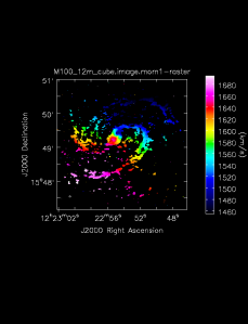
Comparison with 12m alone Moment Maps
Below the moment maps from the 12m alone data are shown for comparison. The range and scaling are the same as that used for the 7m+12m figures. As expected the 7m+12m image shows considerably more extended emission. For comparison the 12m alone synthesized beam is 3.43"x2.38" while the 7m+12m is 3.93"x2.59".
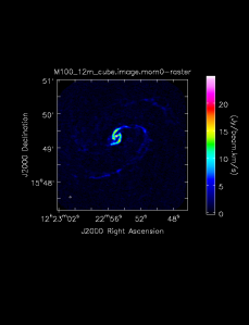
Moment 0 for 12m data alone.
Moment 0 for 12m data alone.


Convert 7m+12m Images to Fits Format
# In CASA
cpaste
exportfits(imagename='M100_Intcombo_0.193_cube.image',fitsimage='M100_Intcombo_0.193_cube.image.fits')

exportfits(imagename='M100_Intcombo_0.193_cube.flux',fitsimage='M100_Intcombo_0.193_cube.flux.fits')

exportfits(imagename='M100_Intcombo_0.193_cube.image.mom0',fitsimage='M100_Intcombo_0.193_cube.image.mom0.fits')

exportfits(imagename='M100_Intcombo_0.193_cube.image.mom0.pbcor',fitsimage='M100_Intcombo_0.193_cube.image.mom0.pbcor.fits')

exportfits(imagename='M100_Intcombo_0.193_cube.image.mom1',fitsimage='M100_Intcombo_0.193_cube.image.mom1.fits')

--
Feathering
Last checked on CASA Version 4.1.0.