M100 Band3 Combine 4.2.2: Difference between revisions
No edit summary |
No edit summary |
||
| Line 1: | Line 1: | ||
= Overview = | = Overview = | ||
= Overview = | |||
= Combine and Image the 7m+12m = | |||
== Split off CO spws == | |||
<source lang="python"> | |||
# In CASA | |||
os.system('m100_*m.ms.listobs') | |||
listobs('M100_Band3_12m_CalibratedData.ms',listfile='m100_12m.ms.listobs') | |||
listobs('M100_Band3_7m_CalibratedData.ms',listfile='m100_7m.ms.listobs') | |||
</source> | |||
<pre style="background-color: #fffacd;"> | |||
</pre> | |||
Investigation shows that the CO is spw=0 for the 12m data and in | |||
spws 1,3 for the 7m data. There are two for the 7m data because some | |||
of the data was taken with a slightly different correlator setup. | |||
Also note that the integration time per visibility is different: | |||
10.1s for the 7m and 6.05s for the 12m data as this will be | |||
important to correctly weighting the data. | |||
<source lang="python"> | |||
# In CASA | |||
os.system('rm -rf m100_12m_CO.ms') | |||
split(vis='M100_Band3_12m_CalibratedData.ms', | |||
outputvis='m100_12m_CO.ms',spw='0',field='M100', | |||
datacolumn='data',keepflags=False) | |||
os.system('rm -rf m100_7m_CO.ms') | |||
split(vis='M100_Band3_7m_CalibratedData.ms', | |||
outputvis='m100_7m_CO.ms',spw='1,3',field='M100', | |||
datacolumn='data',keepflags=False) | |||
</source> | |||
Because the continuum is too weak to contribute to a 5km/s | |||
channel we will forgo the the continuum subtraction step. | |||
== Concat with 1/sigma**2 scaling of Weights == | |||
When combining data with disparate properties it is very important | |||
that the relative weights of each visibility be in the correct | |||
proportion to the other data according to the radiometer equation. | |||
Formally, the | |||
visibility weights should be proportional to 1/sigma**2 where sigma | |||
is the variance or rms noise of a given visibility. | |||
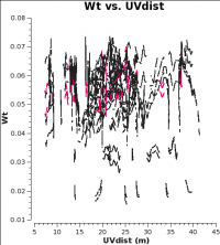
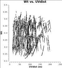
<figure id="12m_WT.png"> | |||
[[File:7m_WT.png|200px|thumb|right|<caption> 12m weights.</caption>]] | |||
</figure> | |||
<figure id="7m_WT.png"> | |||
[[File:12m_WT.png|200px|thumb|right|<caption> 7m weights.</caption>]] | |||
</figure> | |||
CASA currently scales the weights by 1/[(Tsys(i) * Tsys(j)] if | |||
calwt=True for the Tsys table applycal. To verify, we plot the | |||
weights of the 7m and 12m data. No averaging can be turned on | |||
when plotting the weights. | |||
<source lang="python"> | |||
# In CASA | |||
os.system('rm -rf 7m_WT.png 12m_WT.png') | |||
plotms(vis='m100_12m_CO.ms',yaxis='wt',xaxis='uvdist',spw='0~2:200', | |||
coloraxis='spw',plotfile='12m_WT.png') | |||
plotms(vis='m100_7m_CO.ms',yaxis='wt',xaxis='uvdist',spw='0~2:200', | |||
coloraxis='spw',plotfile='7m_WT.png') | |||
</source> | |||
As you can see from these plots, the weights are quite similar at this | |||
stage because the data were taken under similar weather conditions and | |||
hence Tsys. | |||
Assuming that the 7m and 12m antennas have similar apperture and quantization | |||
efficiencies (a reasonable assumption since they were designed this way) | |||
rms noise in a single channel for a single visibility is: | |||
<math> | |||
\sigma_{ij}=\frac{2k}{A_{eff}} | |||
</math> | |||
<math> | |||
\sqrt{\frac{T_{sys,i} T_{sys,j}}{\Delta\nu_{ch} t_{ij}}} | |||
</math> | |||
Where k is Boltzmann's constant, A<sub>eff</sub> is the effective antenna | Where k is Boltzmann's constant, A<sub>eff</sub> is the effective antenna | ||
area, T<sub>sys,i</sub> is the system temperature for | area, T<sub>sys,i</sub> is the system temperature for antenna i, | ||
Δν<sub>ch</sub> is the channel width, and t<sub>ij</sub> | Δν<sub>ch</sub> is the channel width, and t<sub>ij</sub> | ||
is the integration time per visibility. | is the integration time per visibility. | ||
The two key things that are different between the 7m and 12m-array data are | |||
that the effective dish Areas are different by (7/12)**2 and the integration | |||
times are different by sqrt(10.1/6.05). Since dish area is in the numerator of | |||
the radiometer equation and integration time per visibility is in the | |||
denominator, and assuming WT propto 1/sigma**2, | |||
the 7m weight should be scaled by: 7m WT = (7./12.)**4*(10.1/6.05) = 0.193 to | |||
account for the difference in telescope size and integration time | |||
per visibility. | |||
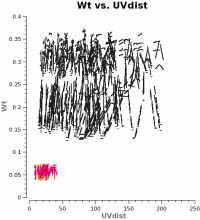
<figure id="Intcombo_0.193_WT.png"> | |||
[[File:Intcombo_0.193_WT.png|200px|thumb|right|<caption> 7m and 12m weights after scaling by relative sensitivity.</caption>]] | |||
</figure> | |||
<source lang="python"> | |||
# In CASA | |||
os.system('rm -rf M100_Intcombo_0.193.ms') | |||
concat(vis=['m100_12m_CO.ms','m100_7m_CO.ms'], | |||
concatvis='M100_Intcombo_0.193.ms', | |||
visweightscale=[1,0.193]) | |||
</source> | |||
<source lang="python"> | |||
# In CASA | |||
os.system('rm -rf Intcombo_0.193_WT.png') | |||
plotms(vis='M100_Intcombo_0.193.ms',yaxis='wt',xaxis='uvdist',spw='0~2:200', | |||
coloraxis='spw',plotfile='Intcombo_0.193_WT.png') | |||
</source> | |||
<source lang="python"> | |||
# In CASA | |||
os.system('rm -rfM100_Intcombo_0.193 _uvdist.png') | |||
plotms(vis='M100_Intcombo_0.193.ms',yaxis='amp',xaxis='uvdist',spw='', | |||
avgchannel='5000', | |||
coloraxis='spw',plotfile='M100_Intcombo_0.193_uvdist.png') | |||
os.system('rm -rfM100_Intcombo_0.193 _vel.png') | |||
plotms(vis='M100_Intcombo_0.193.ms',yaxis='amp',xaxis='velocity',spw='', | |||
avgtime='1e8',coloraxis='spw', | |||
transform=True,freqframe='LSRK',restfreq='115.271201800GHz', | |||
plotfile='M100_Intcombo_0.193_vel.png') | |||
os.system('rm -rfM100_Intcombo_0.193 _chan.png') | |||
plotms(vis='M100_Intcombo_0.193.ms',yaxis='amp',xaxis='channel',spw='', | |||
avgtime='1e8',coloraxis='spw',plotfile='M100_Intcombo_0.193_chan.png') | |||
</source> | |||
Revision as of 15:19, 17 June 2013
Overview
Overview
Combine and Image the 7m+12m
Split off CO spws
# In CASA
os.system('m100_*m.ms.listobs')
listobs('M100_Band3_12m_CalibratedData.ms',listfile='m100_12m.ms.listobs')
listobs('M100_Band3_7m_CalibratedData.ms',listfile='m100_7m.ms.listobs')
Investigation shows that the CO is spw=0 for the 12m data and in spws 1,3 for the 7m data. There are two for the 7m data because some of the data was taken with a slightly different correlator setup.
Also note that the integration time per visibility is different: 10.1s for the 7m and 6.05s for the 12m data as this will be important to correctly weighting the data.
# In CASA
os.system('rm -rf m100_12m_CO.ms')
split(vis='M100_Band3_12m_CalibratedData.ms',
      outputvis='m100_12m_CO.ms',spw='0',field='M100',
      datacolumn='data',keepflags=False)
os.system('rm -rf m100_7m_CO.ms')
split(vis='M100_Band3_7m_CalibratedData.ms',
      outputvis='m100_7m_CO.ms',spw='1,3',field='M100',
      datacolumn='data',keepflags=False)
Because the continuum is too weak to contribute to a 5km/s channel we will forgo the the continuum subtraction step.
Concat with 1/sigma**2 scaling of Weights
When combining data with disparate properties it is very important that the relative weights of each visibility be in the correct proportion to the other data according to the radiometer equation. Formally, the visibility weights should be proportional to 1/sigma**2 where sigma is the variance or rms noise of a given visibility.
<figure id="12m_WT.png">
</figure>
<figure id="7m_WT.png">
</figure>
CASA currently scales the weights by 1/[(Tsys(i) * Tsys(j)] if
calwt=True for the Tsys table applycal. To verify, we plot the
weights of the 7m and 12m data. No averaging can be turned on
when plotting the weights.
# In CASA
os.system('rm -rf 7m_WT.png 12m_WT.png')
plotms(vis='m100_12m_CO.ms',yaxis='wt',xaxis='uvdist',spw='0~2:200',
       coloraxis='spw',plotfile='12m_WT.png')

plotms(vis='m100_7m_CO.ms',yaxis='wt',xaxis='uvdist',spw='0~2:200',
       coloraxis='spw',plotfile='7m_WT.png')
As you can see from these plots, the weights are quite similar at this stage because the data were taken under similar weather conditions and hence Tsys.
Assuming that the 7m and 12m antennas have similar apperture and quantization efficiencies (a reasonable assumption since they were designed this way)
rms noise in a single channel for a single visibility is:
[math]\displaystyle{ \sigma_{ij}=\frac{2k}{A_{eff}} }[/math] [math]\displaystyle{ \sqrt{\frac{T_{sys,i} T_{sys,j}}{\Delta\nu_{ch} t_{ij}}} }[/math]
Where k is Boltzmann's constant, Aeff is the effective antenna
area, Tsys,i is the system temperature for antenna i,
Δνch is the channel width, and tij
is the integration time per visibility.
The two key things that are different between the 7m and 12m-array data are that the effective dish Areas are different by (7/12)**2 and the integration times are different by sqrt(10.1/6.05). Since dish area is in the numerator of the radiometer equation and integration time per visibility is in the denominator, and assuming WT propto 1/sigma**2, the 7m weight should be scaled by: 7m WT = (7./12.)**4*(10.1/6.05) = 0.193 to account for the difference in telescope size and integration time per visibility.
<figure id="Intcombo_0.193_WT.png">
</figure>
# In CASA
os.system('rm -rf M100_Intcombo_0.193.ms')
concat(vis=['m100_12m_CO.ms','m100_7m_CO.ms'],
       concatvis='M100_Intcombo_0.193.ms',
       visweightscale=[1,0.193])
# In CASA
os.system('rm -rf Intcombo_0.193_WT.png')
plotms(vis='M100_Intcombo_0.193.ms',yaxis='wt',xaxis='uvdist',spw='0~2:200',
       coloraxis='spw',plotfile='Intcombo_0.193_WT.png')
# In CASA
os.system('rm -rfM100_Intcombo_0.193 _uvdist.png')
plotms(vis='M100_Intcombo_0.193.ms',yaxis='amp',xaxis='uvdist',spw='',
       avgchannel='5000',
       coloraxis='spw',plotfile='M100_Intcombo_0.193_uvdist.png')

os.system('rm -rfM100_Intcombo_0.193 _vel.png')
plotms(vis='M100_Intcombo_0.193.ms',yaxis='amp',xaxis='velocity',spw='',
       avgtime='1e8',coloraxis='spw',
       transform=True,freqframe='LSRK',restfreq='115.271201800GHz',
       plotfile='M100_Intcombo_0.193_vel.png')

os.system('rm -rfM100_Intcombo_0.193 _chan.png')
plotms(vis='M100_Intcombo_0.193.ms',yaxis='amp',xaxis='channel',spw='',
       avgtime='1e8',coloraxis='spw',plotfile='M100_Intcombo_0.193_chan.png')


