JVLA - Priori Flagging, Auto-Flagging, and Imaging in CASA: Difference between revisions
No edit summary |
No edit summary |
||
| Line 42: | Line 42: | ||
</source> | </source> | ||
This should take several minutes, but once it's complete, you will have a directory called SNR_G55_10s.ms <font color=green>(6.1GB)</font> and SNR_G55_10s.pos, which are the MS (Measurement Set) and antenna position | This should take several minutes, but once it's complete, you will have a directory called SNR_G55_10s.ms <font color=green>(6.1GB)</font> and SNR_G55_10s.pos, which are the MS (Measurement Set) and an antenna position correction. | ||
The antenna position | The antenna position correction was generated using gencal:<br /> | ||
''gencal(vis='SNR_G55_10s.ms', caltable='SNR_G55_10s.pos', caltype='antpos')'' | ''gencal(vis='SNR_G55_10s.ms', caltable='SNR_G55_10s.pos', caltype='antpos')'' | ||
In order to save time, we've included | In order to save time, we've included it in the tar file and will be applying it later in the tutorial. | ||
== Starting CASA 4.5.2 == | == Starting CASA 4.5.2 == | ||
| Line 365: | Line 365: | ||
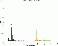
Let's create before and after images with the {{plotms}} task, to see the effects of hanning-smoothing the data. | Let's create before and after images with the {{plotms}} task, to see the effects of hanning-smoothing the data. | ||
[[Image:amp_v_freq_before_after_hanning.gif|200px|thumb|right|The effects of applying Hanning-Smoothing to our data]] | |||
<source lang="python"> | <source lang="python"> | ||
| Line 445: | Line 447: | ||
The logger will report that almost 28.5% of the table selection has been flagged. This makes sense since this spectral window didn't show much of the RFI present in spectral window 0. Let us now run tfcrop on the two remaining spectral windows, 2 and 3. | The logger will report that almost 28.5% of the table selection has been flagged. This makes sense since this spectral window didn't show much of the RFI present in spectral window 0. Let us now run tfcrop on the two remaining spectral windows, 2 and 3. | ||
''' spw 2 & 3 ''' | ''' spw 2 & 3 ''' | ||
| Line 461: | Line 461: | ||
display='', flagbackup=False) | display='', flagbackup=False) | ||
</source> | </source> | ||
[[Image:amp_v_freq_before_after_tfcrop_scan190.gif|200px|thumb|right|The effects of applying tfcrop to our data, for scan 190.]] | |||
We can now use {{plotms}} to review the effects of using tfcrop and compare the image to the one created before applying tfcrop. We can see great improvements, especially for spectral window 0 and 2, which had some of the worst RFI. | We can now use {{plotms}} to review the effects of using tfcrop and compare the image to the one created before applying tfcrop. We can see great improvements, especially for spectral window 0 and 2, which had some of the worst RFI. | ||
| Line 485: | Line 487: | ||
</source> | </source> | ||
The results indicate we have flagged | The results indicate we have flagged a little over 17% of G55.7+3.4. We can now move on to the other auto-flagging algorithm, rflag. | ||
=== RFlag === | === RFlag === | ||
| Line 506: | Line 508: | ||
<pre> | <pre> | ||
SPW 0: | SPW 0: 19-21 | ||
SPW 1: 30-33 | SPW 1: 30-33 | ||
SPW 2: 32-35 | SPW 2: 32-35 | ||
| Line 517: | Line 519: | ||
# In CASA | # In CASA | ||
gaincal(vis='SNR_G55_10s.ms', caltable='SNR_G55_10s.initPh', field='J1925+2106', solint='int', | gaincal(vis='SNR_G55_10s.ms', caltable='SNR_G55_10s.initPh', field='J1925+2106', solint='int', | ||
spw='0: | spw='0:19~21,1;3:30~33,2:32~35', refant='ea24', minblperant=3, | ||
minsnr=3.0, calmode='p', gaintable='SNR_G55_10s.pos') | minsnr=3.0, calmode='p', gaintable='SNR_G55_10s.pos') | ||
</source> | </source> | ||
| Line 531: | Line 533: | ||
* gaintable='SNR_G55_10s.pos': use the antenna position correction for ea07 that we included in the tar file. | * gaintable='SNR_G55_10s.pos': use the antenna position correction for ea07 that we included in the tar file. | ||
Note that a number of solutions do not pass the requirements of the minimum 3 baselines (generating the terminal message "Insufficient unflagged antennas to proceed with this solve.") or minimum signal-to-noise ratio (outputting "n of x solutions rejected due to SNR < 3 ..."). | Note that a number of solutions do not pass the requirements of the minimum 3 baselines (generating the terminal message "Insufficient unflagged antennas to proceed with this solve.") or minimum signal-to-noise ratio (outputting "n of x solutions rejected due to SNR < 3 ..."). The logger output indicates 348 solutions succeeded, out of 387 attempted. | ||
[[Image: | [[Image:gainPh_vs_time_ea10.png|200px|thumb|right| Gain Phase vs. Time for ea10, spectral window 0.]] | ||
[[Image:gainPh_vs_time_spw2.png|200px|thumb|right| Gain Phase vs. Time for spw2 with a subset of antennas.]] | |||
It's always a good idea to inspect the resulting calibration table with {{plotcal}}. | |||
<source lang="python"> | <source lang="python"> | ||
# In CASA | # In CASA | ||
plotcal(caltable='SNR_G55_10s.initPh', xaxis='time', yaxis='phase', iteration=' | plotcal(caltable='SNR_G55_10s.initPh', xaxis='time', yaxis='phase', iteration='antenna', | ||
spw='0', plotrange=[-1,-1,-180,180]) | |||
</source> | </source> | ||
This will iterate over several antennas. We can see that the phase does not change much over the course of the observation for spw 0. Let's now iterate over the spectral windows for a few of the antennas. | |||
<source lang="python"> | |||
# In CASA | |||
plotcal(caltable='SNR_G55_10s.initPh', xaxis='time', yaxis='phase', iteration='spw', | |||
antenna='ea01,ea05,ea10,ea24', plotrange=[-1,-1,-180,180]) | |||
</source> | |||
Now that we've determined our plots look fairly reasonable | Now that we've determined our plots look fairly reasonable, we will create a time-averaged bandpass solutions for the phase calibration source using the {{bandpass}} task. | ||
<source lang="python"> | <source lang="python"> | ||
| Line 562: | Line 569: | ||
Again, we can see that a number of solutions have been rejected by our choice of <tt>minsnr</tt>. | Again, we can see that a number of solutions have been rejected by our choice of <tt>minsnr</tt>. | ||
[[Image: | [[Image:GainAmp_vs_Freq_bandpass.png|200px|thumb|right|Bandpasses for antennas ea20 - ea28]] | ||
Let us now inspect the resulting bandpass plots with plotcal. | |||
<source lang="python"> | <source lang="python"> | ||
| Line 574: | Line 581: | ||
* subplot=331: displays 3x3 plots per screen | * subplot=331: displays 3x3 plots per screen | ||
We will apply these calibration tables using {{applycal}}. | |||
<source lang="python"> | <source lang="python"> | ||
Revision as of 19:09, 14 March 2016
- Topical guide, part 1 of 2.
- This CASA guide is designed for CASA 4.5.2
- **This guide is under construction**
Overview
This CASA guide will cover priori data flagging, including online flagging, shadowing, zero clipping, and quacking. We will then move on to auto-flagging RFI via tfcrop and rflag.
Part 2 of the guide covers advanced imaging, including Multi-Scale, MS-MFS, W/AW-Projection, widefield, outlier fields, spectral index imaging, and imaging in interactive mode. Other topics include primary beam corrections, small scale bias, and weighting.
We will be utilizing data taken with the Karl G. Jansky, Very Large Array, of a supernova remnant G055.7+3.4.. The data were taken on August 23, 2010, in the first D-configuration for which the new wide-band capabilities of the WIDAR (Wideband Interferometric Digital ARchitecture) correlator were available. The 8-hour-long observation includes all available 1 GHz of bandwidth in L-band, from 1-2 GHz in frequency.
Obtaining the Data
A copy of the data (5.1GB) can be downloaded here: ###PROVIDE LINK###
For convenience, we will start with this data set that has been imported using importasdm().
importasdm(asdm='AB1345_sb1800808_1.55431.004049953706', vis='SNR_G55.ms', process_flags=True, tbuff=1.5, applyflags=False, outfile='SNR_G55.ms.onlineflags.txt', flagbackup=False)
- process_flags=True: This parameter controls the creation of online flags from the Flag.xml SDM table. It will create online flags in the FLAG_CMD sub-table within the MS (more on this later).
- tbuff=1.5: This parameter adds a time "buffer" padding to the flags in both directions to deal with timing mismatches. This is important for JVLA data taken before April 2011. This value should be set to 1.5x integration time. This particular observation had 1 second integrations. (CASA Cookbook section 2.2.2 and 3.5.1.3)
- applyflags=False: We will apply these flags later in the tutorial.
- outfile='SNR_G55.ms.onlineflags.txt': This will create a text file with a list of online flags that can be applied. Created just for convenience, and won't be used during the tutorial.
Split and time-averaged using the new task split2() task which uses the mstransform() framework. Please note that split2 will be replacing split in future CASA releases.
split2(vis='SNR_G55.ms', outputvis='SNR_G55_10s.ms', field='3~5', spw='4~5,7~8', antenna='!ea06,ea17,ea20,ea26', datacolumn='data', keepflags=False, timebin='10s')
- field: Several fields have been removed which we won't be utilizing. Only keeping fields 3-5.
- spw: Several spectral windows have been removed which were polluted with RFI, which neither auto-flagging nor hand flagging could remedy. Keeping spectral windows 4,5,7,8.
- antenna: Several antennas have been removed (!), which at the time of the observation, didn't have an L-Band receiver installed. (more on this later)
- Time-averaged to 10-seconds, to reduce size and processing time when running tasks.
The original data set is roughly (170GB) in size, and can be downloaded from the NRAO Science Data Archive. The archive file name is AB1345_sb1800808_1.55431.004049953706. Note that within the archive, you can also request specific scans which can be time averaged, with online flags applied.
Once you've downloaded the file, let's untar it:
tar -xzvf SNR_G55_10s.tar.gz
This should take several minutes, but once it's complete, you will have a directory called SNR_G55_10s.ms (6.1GB) and SNR_G55_10s.pos, which are the MS (Measurement Set) and an antenna position correction.
The antenna position correction was generated using gencal:
gencal(vis='SNR_G55_10s.ms', caltable='SNR_G55_10s.pos', caltype='antpos')
In order to save time, we've included it in the tar file and will be applying it later in the tutorial.
Starting CASA 4.5.2
Start CASA by typing casa on a terminal command line. If you have not used CASA before, some helpful tips are available on the Getting Started in CASA page.
This guide has been written for CASA version 4.5.2. Please confirm your version before proceeding by checking the message in the command line interface window or the CASA logger after startup.
For this tutorial, we will be running tasks using the task (parameter = value) syntax. When called in this manner, all parameters not explicitly set will use their default values.
Preliminary Data Evaluation
As a first step, use listobs to have a look at the MS:
# In CASA
listobs(vis='SNR_G55_10s.ms', listfile='SNR_G55_10s.listobs')
- listfile: Creates a text document with details for the observation.
#CASA log when listfile is not defined
2016-03-07 16:54:23 INFO listobs  ##########################################
2016-03-07 16:54:23 INFO listobs  ##### Begin Task: listobs            #####
2016-03-07 16:54:23 INFO listobs  listobs(vis="SNR_G55_10s.ms",selectdata=True,spw="",field="",antenna="",
2016-03-07 16:54:23 INFO listobs	  uvrange="",timerange="",correlation="",scan="",intent="",
2016-03-07 16:54:23 INFO listobs	  feed="",array="",observation="",verbose=True,listfile="",
2016-03-07 16:54:23 INFO listobs	  listunfl=False,cachesize=50,overwrite=False)
2016-03-07 16:54:23 INFO listobs  ================================================================================
2016-03-07 16:54:23 INFO listobs	     MeasurementSet Name:  /lustre/aoc/sciops/CASA_Tutorials/SNR_G55_10s.ms      MS Version 2
2016-03-07 16:54:23 INFO listobs  ================================================================================
2016-03-07 16:54:23 INFO listobs     Observer: Dr. Sanjay Sanjay Bhatnagar     Project: uid://evla/pdb/1072564
2016-03-07 16:54:23 INFO listobs  Observation: EVLA
2016-03-07 16:54:25 INFO listobs  Data records: 3780000       Total elapsed time = 26926 seconds
2016-03-07 16:54:25 INFO listobs     Observed from   23-Aug-2010/00:56:36.0   to   23-Aug-2010/08:25:22.0 (UTC)
2016-03-07 16:54:33 INFO listobs
2016-03-07 16:54:33 INFO listobs     ObservationID = 0         ArrayID = 0
2016-03-07 16:54:33 INFO listobs  Date        Timerange (UTC)          Scan  FldId FieldName    nRows     SpwIds       Average Interval(s)    ScanIntent
2016-03-07 16:54:33 INFO listobs  23-Aug-2010/00:56:36.0 - 00:58:06.0    14      0 J1925+2106     12600  [0,1,2,3]  [10, 10, 10, 10, 10] [CALIBRATE_PHASE#UNSPECIFIED]
2016-03-07 16:54:33 INFO listobs	      00:58:06.0 - 00:59:36.0    15      0 J1925+2106     12600  [0,1,2,3]  [10, 10, 10, 10, 10] [CALIBRATE_PHASE#UNSPECIFIED]
2016-03-07 16:54:33 INFO listobs	      00:59:36.0 - 01:01:05.0    16      0 J1925+2106     12600  [0,1,2,3]  [9.89, 9.89, 9.89, 9.89, 9.89] [CALIBRATE_PHASE#UNSPECIFIED]
2016-03-07 16:54:33 INFO listobs	      01:01:05.0 - 01:02:35.0    17      0 J1925+2106     12600  [0,1,2,3]  [10, 10, 10, 10, 10] [CALIBRATE_PHASE#UNSPECIFIED]
2016-03-07 16:54:33 INFO listobs	      01:02:35.0 - 01:04:05.0    18      0 J1925+2106     12600  [0,1,2,3]  [10, 10, 10, 10, 10] [CALIBRATE_PHASE#UNSPECIFIED]
2016-03-07 16:54:33 INFO listobs	      01:04:05.0 - 01:05:34.0    19      0 J1925+2106     12600  [0,1,2,3]  [9.89, 9.89, 9.89, 9.89, 9.89] [CALIBRATE_PHASE#UNSPECIFIED]
2016-03-07 16:54:33 INFO listobs	      01:05:34.0 - 01:07:04.0    20      0 J1925+2106     12600  [0,1,2,3]  [10, 10, 10, 10, 10] [CALIBRATE_PHASE#UNSPECIFIED]
2016-03-07 16:54:33 INFO listobs	      01:07:04.0 - 01:08:34.0    21      1 G55.7+3.4      12600  [0,1,2,3]  [10, 10, 10, 10, 10] [OBSERVE_TARGET#UNSPECIFIED]
2016-03-07 16:54:33 INFO listobs	      01:08:34.0 - 01:10:04.0    22      1 G55.7+3.4      12600  [0,1,2,3]  [10, 10, 10, 10, 10] [OBSERVE_TARGET#UNSPECIFIED]
2016-03-07 16:54:33 INFO listobs	      01:10:04.0 - 01:11:34.0    23      1 G55.7+3.4      12600  [0,1,2,3]  [10, 10, 10, 10, 10] [OBSERVE_TARGET#UNSPECIFIED]
2016-03-07 16:54:33 INFO listobs	      01:11:34.0 - 01:13:03.0    24      1 G55.7+3.4      12600  [0,1,2,3]  [9.89, 9.89, 9.89, 9.89, 9.89] [OBSERVE_TARGET#UNSPECIFIED]
2016-03-07 16:54:33 INFO listobs	      01:13:03.0 - 01:14:33.0    25      1 G55.7+3.4      12600  [0,1,2,3]  [10, 10, 10, 10, 10] [OBSERVE_TARGET#UNSPECIFIED]
2016-03-07 16:54:33 INFO listobs	      01:14:33.0 - 01:16:03.0    26      1 G55.7+3.4      12600  [0,1,2,3]  [10, 10, 10, 10, 10] [OBSERVE_TARGET#UNSPECIFIED]
2016-03-07 16:54:33 INFO listobs	      01:16:03.0 - 01:17:33.0    27      1 G55.7+3.4      12600  [0,1,2,3]  [10, 10, 10, 10, 10] [OBSERVE_TARGET#UNSPECIFIED]
2016-03-07 16:54:33 INFO listobs	      01:17:33.0 - 01:19:02.0    28      1 G55.7+3.4      12600  [0,1,2,3]  [9.89, 9.89, 9.89, 9.89, 9.89] [OBSERVE_TARGET#UNSPECIFIED]
2016-03-07 16:54:33 INFO listobs	      01:19:02.0 - 01:20:32.0    29      1 G55.7+3.4      12600  [0,1,2,3]  [10, 10, 10, 10, 10] [OBSERVE_TARGET#UNSPECIFIED]
2016-03-07 16:54:33 INFO listobs	      01:20:32.0 - 01:22:02.0    30      1 G55.7+3.4      12600  [0,1,2,3]  [10, 10, 10, 10, 10] [OBSERVE_TARGET#UNSPECIFIED]
2016-03-07 16:54:33 INFO listobs	      01:22:02.0 - 01:23:32.0    31      1 G55.7+3.4      12600  [0,1,2,3]  [10, 10, 10, 10, 10] [OBSERVE_TARGET#UNSPECIFIED]
2016-03-07 16:54:33 INFO listobs	      01:23:32.0 - 01:25:01.0    32      1 G55.7+3.4      12600  [0,1,2,3]  [9.89, 9.89, 9.89, 9.89, 9.89] [OBSERVE_TARGET#UNSPECIFIED]
2016-03-07 16:54:33 INFO listobs	      01:25:01.0 - 01:26:31.0    33      1 G55.7+3.4      12600  [0,1,2,3]  [10, 10, 10, 10, 10] [OBSERVE_TARGET#UNSPECIFIED]
2016-03-07 16:54:33 INFO listobs	      01:26:31.0 - 01:28:01.0    34      1 G55.7+3.4      12600  [0,1,2,3]  [10, 10, 10, 10, 10] [OBSERVE_TARGET#UNSPECIFIED]
2016-03-07 16:54:33 INFO listobs	      01:28:01.0 - 01:29:31.0    35      1 G55.7+3.4      12600  [0,1,2,3]  [10, 10, 10, 10, 10] [OBSERVE_TARGET#UNSPECIFIED]
2016-03-07 16:54:33 INFO listobs	      01:29:31.0 - 01:31:00.0    36      1 G55.7+3.4      12600  [0,1,2,3]  [9.89, 9.89, 9.89, 9.89, 9.89] [OBSERVE_TARGET#UNSPECIFIED]
2016-03-07 16:54:33 INFO listobs	      01:31:00.0 - 01:32:30.0    37      1 G55.7+3.4      12600  [0,1,2,3]  [10, 10, 10, 10, 10] [OBSERVE_TARGET#UNSPECIFIED]
2016-03-07 16:54:33 INFO listobs	      01:32:30.0 - 01:34:00.0    38      1 G55.7+3.4      12600  [0,1,2,3]  [10, 10, 10, 10, 10] [OBSERVE_TARGET#UNSPECIFIED]
2016-03-07 16:54:33 INFO listobs	      01:34:00.0 - 01:35:30.0    39      1 G55.7+3.4      12600  [0,1,2,3]  [10, 10, 10, 10, 10] [OBSERVE_TARGET#UNSPECIFIED]
2016-03-07 16:54:33 INFO listobs	      01:35:30.0 - 01:36:59.0    40      1 G55.7+3.4      12600  [0,1,2,3]  [9.89, 9.89, 9.89, 9.89, 9.89] [OBSERVE_TARGET#UNSPECIFIED]
2016-03-07 16:54:33 INFO listobs	      01:36:59.0 - 01:38:29.0    41      0 J1925+2106     12600  [0,1,2,3]  [10, 10, 10, 10, 10] [CALIBRATE_PHASE#UNSPECIFIED]
2016-03-07 16:54:33 INFO listobs	      01:38:29.0 - 01:39:59.0    42      0 J1925+2106     12600  [0,1,2,3]  [10, 10, 10, 10, 10] [CALIBRATE_PHASE#UNSPECIFIED]
2016-03-07 16:54:33 INFO listobs	      01:39:59.0 - 01:41:29.0    43      0 J1925+2106     12600  [0,1,2,3]  [10, 10, 10, 10, 10] [CALIBRATE_PHASE#UNSPECIFIED]
2016-03-07 16:54:33 INFO listobs	      01:41:29.0 - 01:42:58.0    44      1 G55.7+3.4      12600  [0,1,2,3]  [9.89, 9.89, 9.89, 9.89, 9.89] [OBSERVE_TARGET#UNSPECIFIED]
<snip>
2016-03-07 16:54:33 INFO listobs	      08:11:54.0 - 08:13:24.0   305      1 G55.7+3.4      12600  [0,1,2,3]  [10, 10, 10, 10, 10] [OBSERVE_TARGET#UNSPECIFIED]
2016-03-07 16:54:33 INFO listobs	      08:13:24.0 - 08:14:54.0   306      1 G55.7+3.4      12600  [0,1,2,3]  [10, 10, 10, 10, 10] [OBSERVE_TARGET#UNSPECIFIED]
2016-03-07 16:54:33 INFO listobs	      08:14:54.0 - 08:16:24.0   307      2 0542+498=3C147 12600  [0,1,2,3]  [10, 10, 10, 10, 10] [CALIBRATE_AMPLI#UNSPECIFIED,CALIBRATE_BANDPASS#UNSPECIFIED,UNSPECIFIED#UNSPECIFIED]
2016-03-07 16:54:33 INFO listobs	      08:16:24.0 - 08:17:54.0   308      2 0542+498=3C147 12600  [0,1,2,3]  [10, 10, 10, 10, 10] [CALIBRATE_AMPLI#UNSPECIFIED,CALIBRATE_BANDPASS#UNSPECIFIED,UNSPECIFIED#UNSPECIFIED]
2016-03-07 16:54:33 INFO listobs	      08:17:54.0 - 08:19:23.0   309      2 0542+498=3C147 12600  [0,1,2,3]  [9.89, 9.89, 9.89, 9.89, 9.89] [CALIBRATE_AMPLI#UNSPECIFIED,CALIBRATE_BANDPASS#UNSPECIFIED,UNSPECIFIED#UNSPECIFIED]
2016-03-07 16:54:33 INFO listobs	      08:19:23.0 - 08:20:53.0   310      2 0542+498=3C147 12600  [0,1,2,3]  [10, 10, 10, 10, 10] [CALIBRATE_AMPLI#UNSPECIFIED,CALIBRATE_BANDPASS#UNSPECIFIED,UNSPECIFIED#UNSPECIFIED]
2016-03-07 16:54:33 INFO listobs	      08:20:53.0 - 08:22:23.0   311      2 0542+498=3C147 12600  [0,1,2,3]  [10, 10, 10, 10, 10] [CALIBRATE_AMPLI#UNSPECIFIED,CALIBRATE_BANDPASS#UNSPECIFIED,UNSPECIFIED#UNSPECIFIED]
2016-03-07 16:54:33 INFO listobs	      08:22:23.0 - 08:23:52.0   312      2 0542+498=3C147 12600  [0,1,2,3]  [9.89, 9.89, 9.89, 9.89, 9.89] [CALIBRATE_AMPLI#UNSPECIFIED,CALIBRATE_BANDPASS#UNSPECIFIED,UNSPECIFIED#UNSPECIFIED]
2016-03-07 16:54:33 INFO listobs	      08:23:52.0 - 08:25:22.0   313      2 0542+498=3C147 12600  [0,1,2,3]  [10, 10, 10, 10, 10] [CALIBRATE_AMPLI#UNSPECIFIED,CALIBRATE_BANDPASS#UNSPECIFIED,UNSPECIFIED#UNSPECIFIED]
2016-03-07 16:54:33 INFO listobs	           (nRows = Total number of rows per scan)
2016-03-07 16:54:33 INFO listobs  Fields: 3
2016-03-07 16:54:33 INFO listobs   ID   Code Name                RA               Decl           Epoch   SrcId      nRows
2016-03-07 16:54:33 INFO listobs   0    D    J1925+2106          19:25:59.605371 +21.06.26.16218 J2000   0         541800
2016-03-07 16:54:33 INFO listobs   1    NONE G55.7+3.4           19:21:40.000000 +21.45.00.00000 J2000   1        3150000
2016-03-07 16:54:33 INFO listobs   2    N    0542+498=3C147      05:42:36.137916 +49.51.07.23356 J2000   2          88200
2016-03-07 16:54:33 INFO listobs  Spectral Windows:  (5 unique spectral windows and 1 unique polarization setups)
2016-03-07 16:54:33 INFO listobs   SpwID  Name      #Chans   Frame   Ch0(MHz)  ChanWid(kHz)  TotBW(kHz) CtrFreq(MHz) BBC Num  Corrs
2016-03-07 16:54:33 INFO listobs   0      Subband:0     64   TOPO    1256.000      2000.000    128000.0   1319.0000        4  RR  RL  LR  LL
2016-03-07 16:54:33 INFO listobs   1      Subband:2     64   TOPO    1384.000      2000.000    128000.0   1447.0000        4  RR  RL  LR  LL
2016-03-07 16:54:33 INFO listobs   2      Subband:1     64   TOPO    1648.000      2000.000    128000.0   1711.0000        8  RR  RL  LR  LL
2016-03-07 16:54:33 INFO listobs   3      Subband:0     64   TOPO    1776.000      2000.000    128000.0   1839.0000        8  RR  RL  LR  LL
2016-03-07 16:54:33 INFO listobs  Sources: 15
2016-03-07 16:54:33 INFO listobs   ID   Name                SpwId RestFreq(MHz)  SysVel(km/s)
2016-03-07 16:54:33 INFO listobs   0    J1925+2106          0     -              -
2016-03-07 16:54:33 INFO listobs   0    J1925+2106          1     -              -
2016-03-07 16:54:33 INFO listobs   0    J1925+2106          2     -              -
2016-03-07 16:54:33 INFO listobs   0    J1925+2106          3     -              -
2016-03-07 16:54:33 INFO listobs   1    G55.7+3.4           0     -              -
2016-03-07 16:54:33 INFO listobs   1    G55.7+3.4           1     -              -
2016-03-07 16:54:33 INFO listobs   1    G55.7+3.4           2     -              -
2016-03-07 16:54:33 INFO listobs   1    G55.7+3.4           3     -              -
2016-03-07 16:54:33 INFO listobs   2    0542+498=3C147      0     -              -
2016-03-07 16:54:33 INFO listobs   2    0542+498=3C147      1     -              -
2016-03-07 16:54:33 INFO listobs   2    0542+498=3C147      2     -              -
2016-03-07 16:54:33 INFO listobs   2    0542+498=3C147      3     -              -
2016-03-07 16:54:34 INFO listobs  Antennas: 27:
2016-03-07 16:54:34 INFO listobs   ID   Name  Station   Diam.    Long.         Lat.                Offset from array center (m)                ITRF Geocentric coordinates (m)
2016-03-07 16:54:34 INFO listobs                                                                East       North    Elevation        x               y               z
2016-03-07 16:54:34 INFO listobs   0    ea01  W09       25.0 m   -107.37.25.2  +33.53.51.0   -521.9416   -332.7766    -1.2001 -1601710.017000 -5042006.925200  3554602.355600
2016-03-07 16:54:34 INFO listobs   1    ea02  E02       25.0 m   -107.37.04.4  +33.54.01.1      9.8240    -20.4293    -2.7806 -1601150.060300 -5042000.619800  3554860.729400
2016-03-07 16:54:34 INFO listobs   2    ea03  E09       25.0 m   -107.36.45.1  +33.53.53.6    506.056    -251.8670    -3.5825 -1600715.950800 -5042273.187000  3554668.184500
2016-03-07 16:54:34 INFO listobs   3    ea04  W01       25.0 m   -107.37.05.9  +33.54.00.5    -27.3562    -41.3030    -2.7418 -1601189.030140 -5042000.493300  3554843.425700
2016-03-07 16:54:34 INFO listobs   4    ea05  W08       25.0 m   -107.37.21.6  +33.53.53.0   -432.1167   -272.1478    -1.5054 -1601614.091000 -5042001.652900  3554652.509300
2016-03-07 16:54:34 INFO listobs   5    ea06  N06       25.0 m   -107.37.06.9  +33.54.10.3    -54.0649    263.8778    -4.2273 -1601162.591000 -5041828.999000  3555095.896400
2016-03-07 16:54:34 INFO listobs   6    ea07  E05       25.0 m   -107.36.58.4  +33.53.58.8    164.9788    -92.8032    -2.5268 -1601014.462000 -5042086.252000  3554800.799800
2016-03-07 16:54:34 INFO listobs   7    ea08  N01       25.0 m   -107.37.06.0  +33.54.01.8    -30.8810     -1.4664    -2.8597 -1601185.634945 -5041978.156586  3554876.424700
2016-03-07 16:54:34 INFO listobs   8    ea09  E06       25.0 m   -107.36.55.6  +33.53.57.7    236.9058   -126.3369    -2.4443 -1600951.588000 -5042125.911000  3554773.012300
2016-03-07 16:54:34 INFO listobs   9    ea10  N03       25.0 m   -107.37.06.3  +33.54.04.8    -39.0773     93.0192    -3.3330 -1601177.376760 -5041925.073200  3554954.584100
2016-03-07 16:54:34 INFO listobs   10   ea11  E04       25.0 m   -107.37.00.8  +33.53.59.7    102.8054    -63.7682    -2.6414 -1601068.790300 -5042051.910200  3554824.835300
2016-03-07 16:54:34 INFO listobs   11   ea12  E08       25.0 m   -107.36.48.9  +33.53.55.1    407.8285   -206.0065    -3.2272 -1600801.926000 -5042219.366500  3554706.448200
2016-03-07 16:54:34 INFO listobs   12   ea13  N07       25.0 m   -107.37.07.2  +33.54.12.9    -61.1037    344.2331    -4.6138 -1601155.635800 -5041783.843800  3555162.374100
2016-03-07 16:54:34 INFO listobs   13   ea15  W06       25.0 m   -107.37.15.6  +33.53.56.4   -275.8288   -166.7451    -2.0590 -1601447.198000 -5041992.502500  3554739.687600
2016-03-07 16:54:34 INFO listobs   14   ea16  W02       25.0 m   -107.37.07.5  +33.54.00.9    -67.9687    -26.5614    -2.7175 -1601225.255200 -5041980.383590  3554855.675000
2016-03-07 16:54:34 INFO listobs   15   ea17  W07       25.0 m   -107.37.18.4  +33.53.54.8   -349.9877   -216.7509    -1.7975 -1601526.387300 -5041996.840100  3554698.327400
2016-03-07 16:54:34 INFO listobs   16   ea18  N09       25.0 m   -107.37.07.8  +33.54.19.0    -77.4346    530.6273    -5.5859 -1601139.485100 -5041679.036800  3555316.533200
2016-03-07 16:54:34 INFO listobs   17   ea19  W04       25.0 m   -107.37.10.8  +33.53.59.1   -152.8599    -83.8054    -2.4614 -1601315.893000 -5041985.320170  3554808.304600
2016-03-07 16:54:34 INFO listobs   18   ea20  N05       25.0 m   -107.37.06.7  +33.54.08.0    -47.8454    192.6015    -3.8723 -1601168.786100 -5041869.054000  3555036.936000
2016-03-07 16:54:34 INFO listobs   19   ea21  E01       25.0 m   -107.37.05.7  +33.53.59.2    -23.8638    -81.1510    -2.5851 -1601192.467800 -5042022.856800  3554810.438800
2016-03-07 16:54:34 INFO listobs   20   ea22  N04       25.0 m   -107.37.06.5  +33.54.06.1    -42.6239    132.8436    -3.5494 -1601173.979400 -5041902.657700  3554987.517500
2016-03-07 16:54:34 INFO listobs   21   ea23  E07       25.0 m   -107.36.52.4  +33.53.56.5    318.0509   -164.1850    -2.6957 -1600880.571400 -5042170.388000  3554741.457400
2016-03-07 16:54:34 INFO listobs   22   ea24  W05       25.0 m   -107.37.13.0  +33.53.57.8   -210.0959   -122.3887    -2.2577 -1601377.009500 -5041988.665500  3554776.393400
2016-03-07 16:54:34 INFO listobs   23   ea25  N02       25.0 m   -107.37.06.2  +33.54.03.5    -35.6245     53.1806    -3.1345 -1601180.861480 -5041947.453400  3554921.628700
2016-03-07 16:54:34 INFO listobs   24   ea26  W03       25.0 m   -107.37.08.9  +33.54.00.1   -105.3447    -51.7177    -2.6037 -1601265.153600 -5041982.533050  3554834.858400
2016-03-07 16:54:34 INFO listobs   25   ea27  E03       25.0 m   -107.37.02.8  +33.54.00.5     50.6641    -39.4835    -2.7273 -1601114.365500 -5042023.151800  3554844.944000
2016-03-07 16:54:34 INFO listobs   26   ea28  N08       25.0 m   -107.37.07.5  +33.54.15.8    -68.9057    433.1889    -5.0602 -1601147.940400 -5041733.837000  3555235.956000
2016-03-07 16:54:34 INFO listobs ##### End Task: listobs              #####
2016-03-07 16:54:34 INFO listobs ##########################################
- J1925+2106, field ID 0: Phase Calibrator;
- G55.7+3.4, field ID 1: The Supernova Remnant;
- 0542+498=3C147, field ID 2: Amplitude/Bandpass Calibrator
We can also see that these sources have associated "scan intents", which indicate their function in the observation. Note that you can select sources based on their intents in certain CASA tasks. The various scan intents in this data set are:
- CALIBRATE_PHASE indicates that this is a scan to be used for gain calibration;
- OBSERVE_TARGET indicates that this is the science target;
- CALIBRATE_AMPLI indicates that this is to be used for flux calibration; and
- CALIBRATE_BANDPASS indicates that these scans are to be used for bandpass calibration.
Note that 3C147 is to be used for both flux and bandpass calibration.
It's important to also note that the antennas have a name and ID associated with them. For example antenna ID 15 is named ea17 ( The "ea" stemming from the Expanded VLA project). When specifying an antenna within a task parameter, we will mainly reference them by name.
We can see the antenna configuration for this observation by using plotants:
# In CASA
plotants(vis='SNR_G55_10s.ms', figfile='SNR_G55_10s.plotants.png')
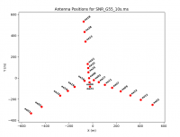
This shows that antennas ea01, ea03, and ea18 were on the extreme ends of the west, east, and north arms, respectively. The antenna position diagram is particularly useful as a guide to help determine which antenna to use as the reference antenna later during calibration. Note that antennas on stations 8 of each arm (N08, E08, W08) do not get moved during array reconfigurations, they can therefore at times be good choices as reference antennas. In this case, we'll probably want to choose something closer to the center of the array.
We may also inspect the raw data using plotms. To start with, lets look at a subset of scans on the supernova remnant:
# In CASA
plotms(vis='SNR_G55_10s.ms', scan='30,75,120,165,190,235,303', antenna='ea24', xaxis='freq',
       yaxis='amp', coloraxis='spw', iteraxis='scan', correlation='RR,LL')
- coloraxis='spw': Parameter indicates that a different color will be assigned to each spectral window.
- antenna='ea24' : We chose only information for antenna ea24.
- iteraxis='scan': Parameter tells plotms to display a new plot for each scan.
- correlation='RR,LL': We just want to display the right and left circular polarizations, without the cross-hand terms.
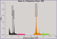
Flipping through to scan 190, we can see that there is significant time and frequency variable RFI present in the observation, as seen by the large spikes in amplitude. In particular, we can see that several spectral windows are quite badly affected. To determine which spectral windows they are, click on the "Mark Regions" tool at the bottom of the plotms GUI (the open box with a green "plus" sign). Use the mouse to select a few of the highest-amplitude points in each of the spectral windows. Click on the "Locate" button (magnifying glass). Information about the selected areas should now display in the logger window:
Frequency in [1.30662 1.31407] or [1.32377 1.33569] or [1.67866 1.69581], Amp in [0.16871 0.217097] or [0.153226 0.186613] or [0.172581 0.235968]:
Scan=190 Field=G55.7+3.4[1] Time=2010/08/23/05:19:58.0 BL=ea16@W02 & ea24@W05[14&22] Spw=0 Chan=27 Freq=1.31  Corr=RR X=1.31  Y=0.17187   (1718/144/1718)
Scan=190 Field=G55.7+3.4[1] Time=2010/08/23/05:19:58.0 BL=ea19@W04 & ea24@W05[17&22] Spw=0 Chan=27 Freq=1.31  Corr=LL X=1.31  Y=0.178607  (1975/144/1975)
Scan=190 Field=G55.7+3.4[1] Time=2010/08/23/05:19:58.0 BL=ea22@N04 & ea24@W05[20&22] Spw=0 Chan=37 Freq=1.33  Corr=RR X=1.33  Y=0.18105   (2250/144/2250)
Scan=190 Field=G55.7+3.4[1] Time=2010/08/23/05:20:08.0 BL=ea19@W04 & ea24@W05[17&22] Spw=0 Chan=27 Freq=1.31  Corr=LL X=1.31  Y=0.21228   (1975/145/1975)
Scan=190 Field=G55.7+3.4[1] Time=2010/08/23/05:20:08.0 BL=ea21@E01 & ea24@W05[19&22] Spw=0 Chan=27 Freq=1.31  Corr=LL X=1.31  Y=0.181632  (2103/145/2103)
Scan=190 Field=G55.7+3.4[1] Time=2010/08/23/05:20:08.0 BL=ea22@N04 & ea24@W05[20&22] Spw=0 Chan=37 Freq=1.33  Corr=RR X=1.33  Y=0.167068  (2250/145/2250)
Scan=190 Field=G55.7+3.4[1] Time=2010/08/23/05:20:28.0 BL=ea19@W04 & ea24@W05[17&22] Spw=0 Chan=27 Freq=1.31  Corr=LL X=1.31  Y=0.216252  (1818323722/147/1975)
Scan=190 Field=G55.7+3.4[1] Time=2010/08/23/05:20:28.0 BL=ea22@N04 & ea24@W05[20&22] Spw=0 Chan=37 Freq=1.33  Corr=RR X=1.33  Y=0.182341  (1818323997/147/2250)
Scan=190 Field=G55.7+3.4[1] Time=2010/08/23/05:20:38.0 BL=ea07@E05 & ea24@W05[6&22]  Spw=0 Chan=27 Freq=1.31  Corr=LL X=1.31  Y=0.175032  (1866691864/148/695)
Scan=190 Field=G55.7+3.4[1] Time=2010/08/23/05:20:38.0 BL=ea09@E06 & ea24@W05[8&22]  Spw=0 Chan=27 Freq=1.31  Corr=RR X=1.31  Y=0.176728  (1866692119/148/950)
Scan=190 Field=G55.7+3.4[1] Time=2010/08/23/05:20:38.0 BL=ea16@W02 & ea24@W05[14&22] Spw=0 Chan=27 Freq=1.31  Corr=LL X=1.31  Y=0.170435  (1866692888/148/1719)
Scan=190 Field=G55.7+3.4[1] Time=2010/08/23/05:20:38.0 BL=ea19@W04 & ea24@W05[17&22] Spw=0 Chan=27 Freq=1.31  Corr=LL X=1.31  Y=0.210123  (1866693144/148/1975)
Scan=190 Field=G55.7+3.4[1] Time=2010/08/23/05:20:38.0 BL=ea21@E01 & ea24@W05[19&22] Spw=0 Chan=27 Freq=1.31  Corr=LL X=1.31  Y=0.185065  (1866693272/148/2103)
Scan=190 Field=G55.7+3.4[1] Time=2010/08/23/05:20:38.0 BL=ea22@N04 & ea24@W05[20&22] Spw=0 Chan=37 Freq=1.33  Corr=RR X=1.33  Y=0.158359  (1866693419/148/2250)
Scan=190 Field=G55.7+3.4[1] Time=2010/08/23/05:20:38.0 BL=ea24@W05 & ea27@E03[22&25] Spw=0 Chan=27 Freq=1.31  Corr=RR X=1.31  Y=0.190659  (1866693783/148/2614)
Scan=190 Field=G55.7+3.4[1] Time=2010/08/23/05:20:48.0 BL=ea21@E01 & ea24@W05[19&22] Spw=0 Chan=27 Freq=1.31  Corr=LL X=1.31  Y=0.197052  (1852669347/149/2103)
Scan=190 Field=G55.7+3.4[1] Time=2010/08/23/05:20:48.0 BL=ea22@N04 & ea24@W05[20&22] Spw=0 Chan=37 Freq=1.33  Corr=RR X=1.33  Y=0.183905  (1852669494/149/2250)
Scan=190 Field=G55.7+3.4[1] Time=2010/08/23/05:20:48.0 BL=ea24@W05 & ea27@E03[22&25] Spw=0 Chan=27 Freq=1.31  Corr=RR X=1.31  Y=0.170542  (1852669858/149/2614)
Scan=190 Field=G55.7+3.4[1] Time=2010/08/23/05:20:58.0 BL=ea21@E01 & ea24@W05[19&22] Spw=0 Chan=27 Freq=1.31  Corr=LL X=1.31  Y=0.179017  (1668509051/150/2103)
Scan=190 Field=G55.7+3.4[1] Time=2010/08/23/05:20:58.0 BL=ea22@N04 & ea24@W05[20&22] Spw=0 Chan=37 Freq=1.33  Corr=RR X=1.33  Y=0.177841  (1668509198/150/2250)
Scan=190 Field=G55.7+3.4[1] Time=2010/08/23/05:21:08.0 BL=ea21@E01 & ea24@W05[19&22] Spw=0 Chan=27 Freq=1.31  Corr=LL X=1.31  Y=0.193158  (1866681459/151/2103)
Scan=190 Field=G55.7+3.4[1] Time=2010/08/23/05:19:58.0 BL=ea19@W04 & ea24@W05[17&22] Spw=2 Chan=19 Freq=1.686 Corr=RR X=1.686 Y=0.209811  (4844192/162/1958)
Scan=190 Field=G55.7+3.4[1] Time=2010/08/23/05:19:58.0 BL=ea19@W04 & ea24@W05[17&22] Spw=2 Chan=19 Freq=1.686 Corr=LL X=1.686 Y=0.224424  (4844193/162/1959)
Scan=190 Field=G55.7+3.4[1] Time=2010/08/23/05:20:08.0 BL=ea19@W04 & ea24@W05[17&22] Spw=2 Chan=19 Freq=1.686 Corr=RR X=1.686 Y=0.231918  (1374179750/163/1958)
Scan=190 Field=G55.7+3.4[1] Time=2010/08/23/05:20:08.0 BL=ea19@W04 & ea24@W05[17&22] Spw=2 Chan=19 Freq=1.686 Corr=LL X=1.686 Y=0.209708  (1374179751/163/1959)
Scan=190 Field=G55.7+3.4[1] Time=2010/08/23/05:20:18.0 BL=ea08@N01 & ea24@W05[7&22]  Spw=2 Chan=19 Freq=1.686 Corr=RR X=1.686 Y=0.17744   (2898499/164/806)
Scan=190 Field=G55.7+3.4[1] Time=2010/08/23/05:20:18.0 BL=ea10@N03 & ea24@W05[9&22]  Spw=2 Chan=19 Freq=1.686 Corr=LL X=1.686 Y=0.177235  (2898756/164/1063)
Scan=190 Field=G55.7+3.4[1] Time=2010/08/23/05:20:18.0 BL=ea19@W04 & ea24@W05[17&22] Spw=2 Chan=19 Freq=1.686 Corr=RR X=1.686 Y=0.230346  (2899651/164/1958)
Scan=190 Field=G55.7+3.4[1] Time=2010/08/23/05:20:18.0 BL=ea19@W04 & ea24@W05[17&22] Spw=2 Chan=19 Freq=1.686 Corr=LL X=1.686 Y=0.199502  (2899652/164/1959)
Scan=190 Field=G55.7+3.4[1] Time=2010/08/23/05:20:28.0 BL=ea08@N01 & ea24@W05[7&22]  Spw=2 Chan=19 Freq=1.686 Corr=RR X=1.686 Y=0.177315  (6083110/165/806)
Scan=190 Field=G55.7+3.4[1] Time=2010/08/23/05:20:28.0 BL=ea10@N03 & ea24@W05[9&22]  Spw=2 Chan=19 Freq=1.686 Corr=LL X=1.686 Y=0.17881   (6083367/165/1063)
Scan=190 Field=G55.7+3.4[1] Time=2010/08/23/05:20:28.0 BL=ea19@W04 & ea24@W05[17&22] Spw=2 Chan=19 Freq=1.686 Corr=RR X=1.686 Y=0.217573  (6084262/165/1958)
Found 45 points (45 unflagged) among 101376 in 0s.
We can see that Spw 0 and 2, are the worst affected by RFI. Also, we get the corresponding frequency where the RFI is present, which looks to be 1.31 and 1.33GHz for spectral window 0, and 1.686GHz for spectral window 2. Visiting the VLA L-Band RFI website, we find that the 1310 and 1330 MHz 'birdies' are due to FAA ASR radars, and the one at 1686MHz is most likely due to a GOES weather satellite. We can compare the plots of the FAA ASR radar from the website, with that of spw 0, and see that the birdies (spikes) are practically identical and fall within the same frequencies.
Priori Calibration and Flagging
Normally, before we proceed with further processing, we should check the operator log for the observation to see if there were any issues noted during the run that need to be addressed. The observing log file for this observation can be found here.
The log has various information, including the start/end times for the observation, frequency bands used, weather, baseline information for recently moved antennas, and any outages or issues that may have been encountered. We can see that antenna ea07 may need position corrections (calibration table SNR_G55_10s.pos will fix this), and several antennas are missing an L-Band receiver, including ea06, ea17, ea20, and ea26. We have already removed these antennas from our MS during the run of split2() and can continue with online flagging.
Online Flags
At the time of importing from the SDM-BDF raw data to a MS, we chose to process the online flags from the Flags.xml file to the FLAG_CMD sub-table within the MS. We also created a txt document which includes a list of online flags.
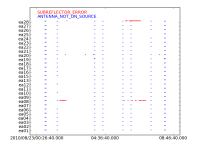
The Flags.xml file holds information of flags created during the observation, such as subreflector issues, and antennas not being on source. We will now want to apply these online flags to the data, but first, let's create a plot of the flags we are about to apply to get an idea of what will be flagged.
We will employ the flagcmd task to apply the online flags.
# In CASA
flagcmd(vis='SNR_G55_10s.ms', inpmode='table', reason='any', action='plot', plotfile='flaggingreason_vs_time.png')
We can see several instances of online flagging in the created image. Most notably, ea28 and ea08 had some subreflector issues througout the observation. Online flags are instances of possible missing data, including:
- ANTENNA_NOT_ON_SOURCE
The JVLA antennas have slewing speeds of 20 degrees per minute in azimuth, and 40 degrees per minute in elevation. Some antennas are slower than others, and may take a few more seconds to reach the next source. The antennas can also take a few seconds to settle down due to small oscillations after having slewed.
- SUBREFLECTOR_ERROR
The FRM (Focus Rotation Mount) located at the apex of the antennas, is responsible for focusing the incoming radio signal to the corresponding receiver. They can at times have issues with their focus and/or rotation axes. Being off target, so much as a few fractions of a degree can result in loss of data, depending on the frequency being observed.
Now that we've plotted the online flags, we will apply them to the MS.
# In CASA
flagcmd(vis='SNR_G55_10s.ms', inpmode='table', reason='any', action='apply', flagbackup=False)
The CASA logger should report the progress as the task applies these flags in chunks. Once it has finished, it will report on the percentage of data that has been flagged.
Shadowed Antennas
Since this is the most compact JVLA configuration, there may be instances where one antenna blocks, or "shadows" another. Therefore, we will run flagdata to remove these data (CASA Cookbook 3.4.2):
# In CASA
flagdata(vis='SNR_G55_10s.ms', mode='shadow', tolerance=0.0, flagbackup=False)
In this particular observation, there does not appear to be much data affected by shadowing, as can be seen in the logger report. One reason why this may be the case, is the antennas were pointed at sources high in elevation.
Zero-Amplitude Data
In addition to shadowing, there may be times during which the correlator writes out pure zero-valued data. In order to remove this bad data, we run flagdata to remove any pure zeroes:
# In CASA
flagdata(vis='SNR_G55_10s.ms', mode='clip', clipzeros=True, flagbackup=False)
Inspecting the logger output which is generated by flagdata shows that there is a small quantity of zero-valued data (4.6%) present in this MS.
Quacking
Now we can utilize the flagdata task one more time in order to run it in quaking mode.
It's common for the array to "settle down" at the start of a scan. Quacking is used to remove data at scan boundaries, and it can apply the same edit to all scans for all baselines. We will forego quacking for this data due to online-flagging having removed the bad data we would otherwise encounter when antennas are not on source. In addition, our science target and phase calibrator J1925+2106 are very close in the sky.
To convince yourself, you can experiment creating a plot of frequency vs. time with plotms for a portion of the observation where the antennas move from the science target, to the phase calibrator. A good choice would be 01:34:00~01:50:27 (scan 39-49).
If we had decided to use the quacking mode, a call to flagdata() would look something like:
flagdata(vis='SN_G55_10s.ms', mode='quack', quackinterval=5.0, quackmode='beg', flagbackup=False)
- quackmode='beg' : Data from the start of each scan will be flagged.
- quackinterval=5.0: Flag the first 5 seconds of every scan.
Backup Data - Flagmanager
Now that we've applied online flags, clipped zero amplitude data, and removed shadowed data, we will create a backup of the MS using flagmanager.
# In CASA
flagmanager(vis='SNR_G55_10s.ms', mode='save', versionname='after_priori_flagging')
From here on forward, if we make a mistake, we can always revert back to this version of the MS by setting mode='restore', and providing the version name we want to restore back to.
Automatic RFI excision
Now that we're done with priori flagging, we can move on to removing some of the RFI present with auto-flagging algorithms used within flagdata. We will employ three CASA tasks, hanningsmooth, flagdata (tfcrop), and flagdata (rflag).
Hanning-Smoothing
Strong RFI sources can give rise to the Gibbs phenomenon. To remedy this ringing across the frequency channels, we can employ the Hanning smoothing algorithm via the hanningsmooth task. Note that running this task overwrites the data, and it cannot be reversed. Also, there is a loss in spectral resolution by a factor of two. In addition, the task allows for the creation of a new MS, or to directly operate on the requested column. For this tutorial, we will be directly operating on the data column.
Let's create before and after images with the plotms task, to see the effects of hanning-smoothing the data.
# In CASA
plotms(vis='SNR_G55_10s.ms', scan='190', antenna='ea24', spw='0~2',
    xaxis='freq', yaxis='amp', coloraxis='spw',
    correlation='RR,LL', plotrange=[1.2,1.8,-0.01,0.25],
    plotfile='amp_v_freq.beforeHanning.png')

hanningsmooth(vis='SNR_G55_10s.ms', datacolumn='data')

plotms(vis='SNR_G55_10s.ms', scan='190', antenna='ea24', spw='0~3',
    xaxis='freq', yaxis='amp', coloraxis='spw',
    correlation='RR,LL', plotrange=[1.2,1.8,-0.01,0.25],
    plotfile='amp_v_freq.afterHanning.png')
Note that the second call to plotms includes a spectral window outside of the plot range. This is to force plotms to reload the plot. By default, plotms will not redraw a plot if the inputs are unchanged. Within the GUI, checking the "reload" box next to the "Plot" button will do this as well.
We can compare the generated plots and take notice that single channel RFI has spread into three channels, but it has also removed some of the worst RFI.
TFcrop
flagdata (tfcrop) is an algorithm that detects outliers in the 2D time-frequency plane, and can operate on un-calibrated data (non bandpass-corrected). Tfcrop will iterate through chunks of time, and undergo several steps in order to find and excise different types of RFI. (CASA Cookbook 3.4.2.7)
Step 1: Detect short-duration RFI spikes (narrow-band and broad-band).
Step 2: Search for time-persistent RFI.
Step 3: Search for time-persistent, narrow-band RFI.
Step 4: Search for low-level wings of very strong RFI.
More details on the algorithm steps can be found on this webpage
We will apply the auto-flagging tfcrop algorithm for each spectral window, one at a time. First, lets plot the corrected data for scan 190, with all spectral windows, so we can compare the data before and after tfcrop.
# In CASA
plotms(vis='SNR_G55_10s.ms', scan='190', antenna='ea24', xaxis='freq', iteraxis='scan',
       yaxis='amp', ydatacolumn='data', plotfile='amp_v_freq_before_tfcrop.png',
       correlation='RR,LL', coloraxis='spw', plotrange=[1.2,2,-0.01,0.25])
Following are a set of flagdata commands which have been found to work reasonably well with these data. Please take some time to play with the parameters and the plotting capabilities. Since these runs set display='both' and action='calculate', the flags are displayed but not actually written to the MS. This allows one to try different sets of parameters before actually applying the flags to the data.
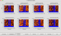
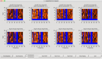
Some representative plots are also displayed. Each column displays an individual polarization product; since we're using all four polarizations, from left to right are RR, RL, LR, and LL. The first row shows the data with current flags applied, and the second includes the flags generated by flagdata. The x-axis is channel number (the spectral window ID is displayed in the top title) and the y-axis of the first two rows is all integrations included in a time "chunk", set by the ntime parameter. These are the data considered by the tfcrop algorithm during its flagging process, and changes in ntime will have some (relatively small) affect on what data are flagged.
Each plot page displays data for a single baseline and time chunk. The buttons at the bottom allow one to step through baseline (backward as well as forward), spw, scan, and field; "Stop Display" will continue the flagging operation without the GUI, and "Quit" aborts the run.
spw 0
# In CASA
flagdata(vis='SNR_G55_10s.ms', mode='tfcrop', spw='0',
         datacolumn='data', action='calculate',
         display='both', flagbackup=False)
As we iterate through the different scans, we can see the flagging we can apply, represented by the blue areas. Let's now apply these flags by changing the action parameter.
# In CASA
flagdata(vis='SNR_G55_10s.ms', mode='tfcrop', spw='0',
         datacolumn='data', action='apply',
         display='', flagbackup=False)
The logger will report that a little over 41% of the table selection has been flagged. We will move on to spectral window 1.
spw 1
# In CASA
flagdata(vis='SNR_G55_10s.ms', mode='tfcrop', spw='1',
         datacolumn='data', action='calculate',
         display='both', flagbackup=False)

flagdata(vis='SNR_G55_10s.ms', mode='tfcrop', spw='1',
         datacolumn='data', action='apply',
         display='', flagbackup=False)
The logger will report that almost 28.5% of the table selection has been flagged. This makes sense since this spectral window didn't show much of the RFI present in spectral window 0. Let us now run tfcrop on the two remaining spectral windows, 2 and 3.
spw 2 & 3
# In CASA

flagdata(vis='SNR_G55_10s.ms', mode='tfcrop', spw='2',
         datacolumn='data', action='apply',
         display='', flagbackup=False)

flagdata(vis='SNR_G55_10s.ms', mode='tfcrop', spw='3',
         datacolumn='data', action='apply',
         display='', flagbackup=False)
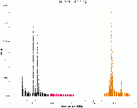
We can now use plotms to review the effects of using tfcrop and compare the image to the one created before applying tfcrop. We can see great improvements, especially for spectral window 0 and 2, which had some of the worst RFI.
# In CASA
plotms(vis='SNR_G55_10s.ms', scan='190', antenna='ea24', xaxis='freq', iteraxis='scan',
       yaxis='amp', ydatacolumn='data', plotfile='amp_v_freq_after_tfcrop.png',
       correlation='RR,LL', coloraxis='spw', plotrange=[1.2,2,-0.01,0.25])
We can now calculate the amount of flagged data so far, in our Measurement Set.
# In CASA
flagInfo = flagdata(vis='SNR_G55_10s.ms', mode='summary')

print("\n %2.1f%% of G55.7+3.4, %2.1f%% of 3C147, and %2.1f%% of J1925+2106 are flagged. \n" % (100.0 * flagInfo['field']['G55.7+3.4']['flagged'] / flagInfo['field']['G55.7+3.4']['total'], 100.0 * flagInfo['field']['0542+498=3C147']['flagged'] / flagInfo['field']['0542+498=3C147']['total'], 100.0 * flagInfo['field']['J1925+2106']['flagged'] / flagInfo['field']['J1925+2106']['total']))

print("Spectral windows are flagged as follows:")

for spw in range(0,4):
     print("SPW %s: %2.1f%%" % (spw, 100.0 * flagInfo['spw'][str(spw)]['flagged'] / flagInfo['spw'][str(spw)]['total']))
The results indicate we have flagged a little over 17% of G55.7+3.4. We can now move on to the other auto-flagging algorithm, rflag.
RFlag
In order to get the best possible result from the automatic RFI excision with flagdata (rflag), we will first apply bandpass calibration to the MS. Since the RFI is time-variable, using the phase calibration source to make an average bandpass over the entire observation will mitigate the amount of RFI present in the calculated bandpass. (For the final calibration, we will use the designated bandpass source 3C147; however, since this object was only observed in the last set of scans, it doesn't sample the time variability and would not provide a good average bandpass.)
Since there are likely to be gain variations over the course of the observation, we will run gaincal to solve for an initial set of antenna-based phases over a narrow range of channels. These will be used to create the bandpass solutions. While amplitude variations will have little effect on the bandpass solutions, it is important to solve for these phase variations with sufficient time resolution to prevent decorrelation when vector averaging the data in computing the bandpass solutions.
In order to choose a narrow range of channels for each spectral window which are relatively RFI-free over the course of the observation, we can look at the data with plotms. Note that it's important to only solve for phase using a narrow channel range, since an antenna-specific delay will cause the phase to vary with respect to frequency over the spectral window, perhaps by a substantial amount.
# In CASA
plotms(vis='SNR_G55_10s.ms', scan='30,75,120,165,190,235,303', antenna='ea24',
       xaxis='channel', yaxis='amp', iteraxis='spw', yselfscale=True, correlation='RR,LL')
- yselfscale=True: sets the y-scaling to be for the currently displayed spectral window, since some spectral windows have much worse RFI and will skew the scale for others.
Looking at these plots, we can choose appropriate channel ranges for each SPW:
SPW 0: 19-21
SPW 1: 30-33
SPW 2: 32-35
SPW 3: 30-33
Using these channel ranges, we run gaincal to calculate phase-only solutions that will be used as input during our initial bandpass calibration. Remember - the calibration tables we are creating now are so that we can use an automatic RFI flagging algorithm. Our final calibration tables will be generated later, after automated flagging. Here are the inputs for our initial pre-bandpass phase calibration:
# In CASA
gaincal(vis='SNR_G55_10s.ms', caltable='SNR_G55_10s.initPh', field='J1925+2106', solint='int',
        spw='0:19~21,1;3:30~33,2:32~35', refant='ea24', minblperant=3,
        minsnr=3.0, calmode='p', gaintable='SNR_G55_10s.pos')
- caltable='SNR_G55_10s.initPh': this is the output calibration table that will be written.
- field='J1925+2106': this is the phase calibrator we will use to calibrate the phases.
- solint='int': we request a solution for each 10-second integration.
- spw='0:11~14,1;3:30~33,2:32~35': note the syntax of this selection: a ":" is used to separate the SPW from channel selection, ";" is used to separate within this selection of spectral windows, and "~" is used to indicate an inclusive range.
- refant='ea24': we have chosen ea24 as the reference antenna after inspecting the antenna position diagram (see above). It is relatively close to, but not directly in, the center of the array, which could be important in D-configuration, since you don't want the reference antenna to have a high probability of being shadowed by nearby antennas.
- minblperant=3: the minimum number of baselines which must be present to attempt a phase solution.
- minsnr=3.0: the minimum signal-to-noise a solution must have to be considered acceptable. Note that solutions which fail this test will cause these data to be flagged downstream of this calibration step.
- calmode='p': perform phase-only solutions.
- gaintable='SNR_G55_10s.pos': use the antenna position correction for ea07 that we included in the tar file.
Note that a number of solutions do not pass the requirements of the minimum 3 baselines (generating the terminal message "Insufficient unflagged antennas to proceed with this solve.") or minimum signal-to-noise ratio (outputting "n of x solutions rejected due to SNR < 3 ..."). The logger output indicates 348 solutions succeeded, out of 387 attempted.
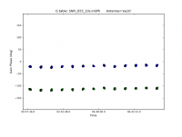
It's always a good idea to inspect the resulting calibration table with plotcal.
# In CASA
plotcal(caltable='SNR_G55_10s.initPh', xaxis='time', yaxis='phase', iteration='antenna',
        spw='0', plotrange=[-1,-1,-180,180])
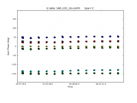
This will iterate over several antennas. We can see that the phase does not change much over the course of the observation for spw 0. Let's now iterate over the spectral windows for a few of the antennas.
# In CASA
plotcal(caltable='SNR_G55_10s.initPh', xaxis='time', yaxis='phase', iteration='spw',
        antenna='ea01,ea05,ea10,ea24', plotrange=[-1,-1,-180,180])
Now that we've determined our plots look fairly reasonable, we will create a time-averaged bandpass solutions for the phase calibration source using the bandpass task.
# In CASA
bandpass(vis='SNR_G55_10s.ms', caltable='SNR_G55_10s.initBP', field='J1925+2106', solint='inf', combine='scan',
         refant='ea24', minblperant=3, minsnr=10.0, gaintable=['SNR_G55_10s.pos', 'SNR_G55_10s.initPh'],
         interp=['', 'nearest'], solnorm=False)
- solint='inf', combine='scan': the solution interval of 'inf' will automatically break by scans; this requests that the solution intervals be combined over scans, so that we will get one solution per antenna.
- gaintable=['SNR_G55_10s.pos', 'SNR_G55_10s.initPh']: we will pre-apply both the antenna position corrections as well as the initial phase solutions.
- interp=['', 'nearest']: by default, gaincal will use linear interpolation for pre-applied calibration. However, we want the nearest phase solution to be used for a given time.
Again, we can see that a number of solutions have been rejected by our choice of minsnr.
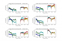
Let us now inspect the resulting bandpass plots with plotcal.
# In CASA
plotcal(caltable='SNR_G55_10s.initBP', xaxis='freq', yaxis='amp',
        iteration='antenna', subplot=331)
- subplot=331: displays 3x3 plots per screen
We will apply these calibration tables using applycal.
# In CASA
applycal(vis='SNR_G55_10s.ms', gaintable=['SNR_G55_10s.pos', 'SNR_G55_10s.initBP'], calwt=False)
This operation will flag data that correspond to flagged solutions, so applycal makes a backup version of the flags prior to operating on the data. Note that running applycal might take a little while.
Now that we have bandpass-corrected data with some RFI flagged out, we will run flagdata in flagdata (rflag) mode (CASA Cookbook 3.4.2.8). Rflag, like tfcrop, is an autoflag algorithm which uses a sliding window statistical filter. Data is iterated through in chunks of time, where statistics are accumulated, and thresholds calculated.
Additional information on the algorithm used in rflag, as well as the statistical details that are undertaken can be found on this webpage (sections 2.1.7).
We will use flagdata with mode='tfcrop', and action='calculate' to first review the amount of data to be flagged. We will also change the datacolumn parameter to 'corrected', since we've applied the bandpass corrections to the MS.
spw 0
# In CASA
flagdata(vis='SNR_G55_10s.ms', mode='rflag', spw='0', datacolumn='corrected',
         action='calculate', display='both', flagbackup=False)
We now run flagdata to calculate and apply these flags for all data in SPW 0. Since this spectral window has more RFI, we are including timedevscale and freqdevscale parameters so as to make the task more sensitive to deviations from the calculated RMS in frequency. The default value is 5.0. Note that this will take a little while.
# In CASA
flagdata(vis='SNR_G55_10s.ms', mode='rflag', spw='0', datacolumn='corrected',
         freqdevscale=2.5, timedevscale=2.5, action='apply', display='both', flagbackup=False)

flagdata(vis='SNR_G55_10s.ms', mode='rflag', spw='0', datacolumn='corrected',
         freqdevscale=2.5, timedevscale=2.5, action='apply', display='', flagbackup=False)
Although RFlag has done a pretty good job of finding the bad data, some still remains. One way to excise the remaining bad data is to use the mode='extend' feature in flagdata, which can extend flags along a chosen axis. First, we will extend the flags across polarization, so if any one polarization is flagged, all data for that time / channel will be flagged:
# In CASA
flagdata(vis='SNR_G55_10s.ms', mode='extend', spw='0', extendpols=True,
         action='apply', display='', flagbackup=False)
Now, we will extend the flags in time and frequency, using the "growtime" and "growfreq" parameters. For the data here, the rflag algorithm seems most likely to miss RFI which should be flagged along more of the time axis, so we will try with growtime=50.0, which will flag all data for a given channel if more than 50% of that channel's time is already flagged, and growfreq=90.0, which will flag the entire spectrum for an integration if more than 90% of the channels in that integration are already flagged.
# In CASA
flagdata(vis='SNR_G55_10s.ms', mode='extend', spw='0', growtime=50.0,
         growfreq=90.0, action='apply', display='', flagbackup=False)
spw 1, 2, and 3
Now, let's work on SPW's 1,2, and 3. We've chosen display='both', in order to first review the flags, and decide if too much or too litle is being flagged. We can always click on 'Quit', and decide to change the freqdevscale and timedevscale parameters, as we did with spectral window 0. Note that spectral window two already has these parameters set, as it contains more RFI.
# In CASA
flagdata(vis='SNR_G55_10s.ms', mode='rflag',  spw='1', datacolumn='corrected',
         freqdevscale=4.0, timedevscale=4.0, action='apply', display='both', flagbackup=False)

flagdata(vis='SNR_G55_10s.ms', mode='extend', spw='1', extendpols=True,
         action='apply', display='', flagbackup=False)

flagdata(vis='SNR_G55_10s.ms', mode='extend', spw='1', growtime=50.0,
         growfreq=90.0, action='apply', display='', flagbackup=False)


flagdata(vis='SNR_G55_10s.ms', mode='rflag',  spw='2', datacolumn='corrected',
         freqdevscale=2.5, timedevscale=2.5, action='apply', display='both', flagbackup=False)

flagdata(vis='SNR_G55_10s.ms', mode='extend', spw='2', extendpols=True,
         action='apply', display='', flagbackup=False)

flagdata(vis='SNR_G55_10s.ms', mode='extend', spw='2', growtime=50.0,
         growfreq=90.0, action='apply', display='', flagbackup=False)


flagdata(vis='SNR_G55_10s.ms', mode='rflag',  spw='3', datacolumn='corrected',
         freqdevscale=4.0, timedevscale=4.0, action='apply', display='both', flagbackup=False)

flagdata(vis='SNR_G55_10s.ms', mode='extend', spw='3', extendpols=True,
         action='apply', display='', flagbackup=False)

flagdata(vis='SNR_G55_10s.ms', mode='extend', spw='3', growtime=50.0,
         growfreq=90.0, action='apply', display='', flagbackup=False)
We can now do as before, and use plotms to see how well rflag has been in removing the RFI.
# In CASA
plotms(vis='SNR_G55_10s.ms', scan='30,75,120,165,190,235,303', xaxis='frequency', yaxis='amp',
ydatacolumn='corrected', iteraxis='scan', correlation='RR,LL', coloraxis = 'spw')
We can also plot amplitude vs. baseline, and look for outliers which we may be able to flag.
# In CASA
plotms(vis='SNR_G55_10s.ms', scan='30,75,120,165,190,235,303', xaxis='baseline', yaxis='amp',
ydatacolumn='corrected', iteraxis='scan', correlation='RR,LL', coloraxis = 'spw')
It appears that there is one baseline which is consistently higher-amplitude than the others, indicating that it's probably contaminated by RFI. Use the plotms tools to identify this baseline, which turns out to be ea04 and ea16, and is mostly present for spw 0 and 1. Let's flag this baseline:
# In CASA
flagdata(vis='SNR_G55_10s.ms', antenna='ea04&ea16', spw='0,1', flagbackup=False)
Let's run flagdata in summary mode, to inspect how much data we have flagged thus far:
# In CASA
flagInfo = flagdata(vis='SNR_G55_10s.ms', mode='summary')

print("\n %2.1f%% of G55.7+3.4, %2.1f%% of 3C147, and %2.1f%% of J1925+2106 are flagged. \n" % (100.0 * flagInfo['field']['G55.7+3.4']['flagged'] / flagInfo['field']['G55.7+3.4']['total'], 100.0 * flagInfo['field']['0542+498=3C147']['flagged'] / flagInfo['field']['0542+498=3C147']['total'], 100.0 * flagInfo['field']['J1925+2106']['flagged'] / flagInfo['field']['J1925+2106']['total']))

print("Spectral windows are flagged as follows:")

for spw in range(0,4):
     print("SPW %s: %2.1f%%" % (spw, 100.0 * flagInfo['spw'][str(spw)]['flagged'] / flagInfo['spw'][str(spw)]['total']))
So, as a result of the flagging, we have sacrificed almost 30% of the data for G55.7+3.4.
Interactive Flagging
After plotting our data, it's obvious that there is still some amount of RFI present. We can use plotms to interactively flag points which look bad. A tutorial on flagging data interactively through plotms can be found here. Please note that flagging data through plotms will not create a backup, so it's important to use the flagmanager before deciding to mark your regions for flagging purposes.
# In CASA
flagmanager(vis='SNR_G55_10s.ms', mode='save',
            versionname='before_interactive_flagging')

# In CASA
plotms(vis='SNR_G55_10s.ms', scan='30,75,120,165,190,235,303',
       xaxis='uvdist', yaxis='amp', iteraxis='spw',
       correlation='RR,LL', coloraxis='antenna1')
Again, nothing really sticks out as obviously in need of flagging. Clearly, there is still some residual RFI left here and there -- however, for the purposes of this tutorial, we will accept the current results and and move on to part two, imaging.
-- original: ??
--modifications: Lorant Sjouwerman (4.4.0, 2015/07/07)
--modifications: Jose Salcido (4.5.1, 2016/02/16)
Last checked on CASA Version 4.5.1.
