JVLA - Basic and Advanced Imaging in CASA: Difference between revisions
No edit summary |
No edit summary |
||
| Line 1: | Line 1: | ||
* '''Topical guide, part 2 of 2''' | * '''Topical guide, part 2 of 2''' | ||
* '''This CASA guide is designed for CASA 4.5. | * '''This CASA guide is designed for CASA 4.5.2''' | ||
| Line 11: | Line 11: | ||
We will be utilizing data taken with the Karl G. Jansky, Very Large Array, of a supernova remnant [http://simbad.u-strasbg.fr/simbad/sim-id?Ident=SNR+G055.7%2B03.4&NbIdent=1&Radius=2&Radius.unit=arcmin&submit=submit+id G055.7+3.4.]. The data were taken on August 23, 2010, in the first D-configuration for which the new wide-band capabilities of the WIDAR (Wideband Interferometric Digital ARchitecture) correlator were available. The 8-hour-long observation includes all available 1 GHz of bandwidth in L-band, from 1-2 GHz in frequency. | We will be utilizing data taken with the Karl G. Jansky, Very Large Array, of a supernova remnant [http://simbad.u-strasbg.fr/simbad/sim-id?Ident=SNR+G055.7%2B03.4&NbIdent=1&Radius=2&Radius.unit=arcmin&submit=submit+id G055.7+3.4.]. The data were taken on August 23, 2010, in the first D-configuration for which the new wide-band capabilities of the WIDAR (Wideband Interferometric Digital ARchitecture) correlator were available. The 8-hour-long observation includes all available 1 GHz of bandwidth in L-band, from 1-2 GHz in frequency. | ||
== Obtaining the | == Obtaining the Data == | ||
We will be utilizing the time-averaged and flagged data from part 1. If you'd like to skip the first part of the tutorial and delve into part 2, you can acquire the measurement set for this tutorial [https://www here]. | We will be utilizing the time-averaged and flagged data from part 1. If you'd like to skip the first part of the tutorial and delve into part 2, you can acquire the measurement set for this tutorial [https://www here]. | ||
| Line 19: | Line 19: | ||
Start CASA by typing '''casa''' on a terminal command line. If you have not used CASA before, some helpful tips are available on the [[Getting Started in CASA]] page. | Start CASA by typing '''casa''' on a terminal command line. If you have not used CASA before, some helpful tips are available on the [[Getting Started in CASA]] page. | ||
This guide has been written for CASA release 4.5. | This guide has been written for CASA release 4.5.2. Please confirm your version before proceeding by checking the message in the command line interface window or the CASA logger after startup. | ||
== Calibrating | == Calibrating Data == | ||
Now that we are satisfied with the RFI excision, we will move on to the calibration stage. | Now that we are satisfied with the RFI excision, we will move on to the calibration stage. | ||
=== | === Flux Density Scale === | ||
Since we will be using 3C147 as the source of the absolute flux scale for this observation, we must first run {{setjy}} to set the appropriate model amplitudes for this source. | Since we will be using 3C147 as the source of the absolute flux scale for this observation, we must first run {{setjy}} to set the appropriate model amplitudes for this source. | ||
| Line 35: | Line 35: | ||
<source lang="python"> | <source lang="python"> | ||
# In CASA | # In CASA | ||
setjy(vis=' | setjy(vis='SNR_G55_10s.ms', listmodels=True) | ||
</source> | </source> | ||
| Line 42: | Line 42: | ||
<source lang="python"> | <source lang="python"> | ||
# In CASA | # In CASA | ||
setjy(vis=' | setjy(vis='SNR_G55_10s.ms', field='0542*', scalebychan=True, model='3C147_L.im') | ||
</source> | </source> | ||
| Line 50: | Line 49: | ||
'''Note:''' The task setjy uses the Perley-Butler 2010 standard by default. Periodically, the flux density scale at the VLA is revised, updated, or expanded. The most recent standard is Perley-Butler 2013, and can be used by explicitly setting standard='Perley-Butler 2013' in the task. See help setjy for more details. | '''Note:''' The task setjy uses the Perley-Butler 2010 standard by default. Periodically, the flux density scale at the VLA is revised, updated, or expanded. The most recent standard is Perley-Butler 2013, and can be used by explicitly setting standard='Perley-Butler 2013' in the task. See help setjy for more details. | ||
=== | === Ionospheric TEC Corrections === | ||
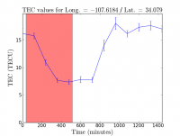
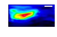
Low frequency observations (4 through S [https://science.nrao.edu/facilities/vla/docs/manuals/oss2013b/performance/bands Bands]) are affected by the ionosphere conditions. A delay can be introduced into the signal path, which is proportional to the Total Electron Content (TEC) along the line of sight, and is inversely proportional to the square of the frequency. We can apply a correction by utilizing GPS measurements taken at two different frequencies from the IGS (International GPS Services) website. We will utilize the {{gencal}} task with paramter caltype set to 'tecim'. This should generate a plot of TEC vs Time for the VLA site, for the day of the observation. | |||
[[Image:TEC_plot.png|200px|thumb|right|Total Electron Content for the VLA site, latitude 34.079, longtitude -107.6184.]] | |||
[[Image:IGS_TEC.gif|200px|thumb|right|Total Electron Content for multiple latitudes and longtitudes.]] | |||
<source lang="python"> | <source lang="python"> | ||
# In CASA | # In CASA | ||
tec_image, tec_rms_image = tec_maps.create(vis='SNR_G55_10s.ms',doplot=True) | |||
gencal(vis='SNR_G55_10s.ms',caltable='SNR_G55_10s.tecim',caltype='tecim',infile=tec_image) | |||
</source> | </source> | ||
The resulting images can be inspected with the CASA {{viewer}} task. As we can see, there was a lot of ionospheric activity on this particular day, therefore applying this correction can result in a better image quality for low-band observing. | |||
=== Delay and Bandpass Calibration === | |||
We will follow a similar procedure as the one outlined in part 1, when we created the preliminary bandpass calibration table SN_G55_10s.initPh. This time, we will use the actual designated bandpass calibration source 0542+498=3C147. Although the phase calibration source used previously (J1925+2106) has the advantage of having been observed throughout the run, it has an unknown spectrum which could introduce amplitude slopes to each spectral window. In addition, we will calibrate the residual antenna-based delays (for further information on this topic, please see this tutorial: [[http://casaguides.nrao.edu/index.php?title=EVLA_3-bit_Tutorial_G192]].) | |||
As before, we first generate a phase-only gain calibration table that will be used to help smooth-out the phases before running {{bandpass}} itself: | |||
<source lang="python"> | <source lang="python"> | ||
# In CASA | # In CASA | ||
gaincal(vis='SNR_G55_10s.ms', field = '2', | |||
caltable='SNR_G55_10s.initPh.2', | |||
spw='*:45~49', solint='int', refant='ea24', | |||
minblperant=3, minsnr=3.0, calmode='p', | |||
gaintable=['SNR_G55_10s.pos', 'SNR_G55_10s.tecim']) | |||
</source> | |||
Again, you will notice a few messages that read "Insufficient unflagged antennas to proceed with this solve." | |||
We can now solve for the residual antenna-based delays that can be seen in plots of the phase vs. frequency for the calibrator sources in {{plotms}}. | We can now solve for the residual antenna-based delays that can be seen in plots of the phase vs. frequency for the calibrator sources in {{plotms}}. | ||
| Line 83: | Line 90: | ||
<source lang="python"> | <source lang="python"> | ||
# In CASA | # In CASA | ||
gaincal(vis=' | gaincal(vis='SNR_G55_10s.ms', field='2', | ||
caltable=' | caltable='SNR_G55_10s.K0', | ||
solint='inf', refant='ea24', | |||
gaintype='K', combine='scan', minsnr=3, | gaintype='K', combine='scan', minsnr=3, | ||
gaintable=[' | gaintable=['SNR_G55_10s.pos', 'SNR_G55_10s.tecim', 'SNR_G55_10s.initPh.2']) | ||
</source> | </source> | ||
We pre-apply our initial phase table, and produce a new K-type caltable for input to bandpass calibration. | We pre-apply our initial phase table, and produce a new K-type caltable for input to bandpass calibration. | ||
We can plot the delays, in nanoseconds, as a function of antenna index (you will get one for each sub-band and polarization): | We can plot the delays, in nanoseconds, as a function of antenna index (you will get one for each sub-band and polarization): | ||
| Line 94: | Line 102: | ||
<source lang="python"> | <source lang="python"> | ||
# In CASA | # In CASA | ||
plotcal(caltable=' | plotcal(caltable='SNR_G55_10s.K0', xaxis='antenna', yaxis='delay') | ||
</source> | </source> | ||
| Line 103: | Line 111: | ||
<source lang="python"> | <source lang="python"> | ||
# In CASA | # In CASA | ||
bandpass(vis=' | bandpass(vis='SNR_G55_10s.ms', caltable='SNR_G55_10s.bPass', | ||
field=' | field='2', solint='inf', combine='scan', | ||
refant='ea24', minblperant=3, minsnr=10.0, | |||
gaintable=[' | gaintable=['SNR_G55_10s.pos', 'SNR_G55_10s.tecim', 'SNR_G55_10s.initPh.2','SNR_G55_10s.K0'], | ||
interp=['', 'nearest', 'nearest'], solnorm=False) | interp=['', 'nearest', 'nearest'], solnorm=False) | ||
</source> | </source> | ||
| Line 119: | Line 127: | ||
<source lang="python"> | <source lang="python"> | ||
# In CASA | # In CASA | ||
plotcal(caltable=' | plotcal(caltable='SNR_G55_10s.bPass', xaxis='freq', yaxis='amp', | ||
iteration='antenna', subplot=331) | iteration='antenna', subplot=331) | ||
# | # | ||
plotcal(caltable=' | plotcal(caltable='SNR_G55_10s.bPass', xaxis='freq', yaxis='phase', | ||
iteration='antenna', subplot=331) | iteration='antenna', subplot=331) | ||
</source> | </source> | ||
| Line 130: | Line 138: | ||
=== Gain calibration === | === Gain calibration === | ||
Next, we will calculate the per-antenna gain solutions. We will now use the intent | Next, we will calculate the per-antenna gain solutions. We will now use the intent parameter. Since this is low-frequency data, we do not expect substantial variations over short timescales, so we calculate one solution per scan (using solint='inf'): | ||
<source lang="python"> | <source lang="python"> | ||
# In CASA | # In CASA | ||
gaincal(vis=' | gaincal(vis='SNR_G55_10s.ms', caltable='SNR_G55_10s.phaseAmp', | ||
intent='*PHASE*,*AMPLI* | intent='*PHASE*,*AMPLI*', solint='inf', refant='ea24', minblperant=3, | ||
minsnr=10.0, gaintable=[' | minsnr=10.0, gaintable=['SNR_G55_10s.pos', 'SNR_G55_10s.tecim', 'SNR_G55_10s.K0','SNR_G55_10s.bPass']) | ||
</source> | </source> | ||
* solint='inf': we request one solution per scan. | * solint='inf': we request one solution per scan. | ||
Plot these solutions as a function of amplitude and phase versus time for the phase calibrator (field | Plot these solutions as a function of amplitude and phase versus time for the phase calibrator (field 0), iterating over each antenna: | ||
<source lang="python"> | <source lang="python"> | ||
# In CASA | # In CASA | ||
plotcal(caltable=' | plotcal(caltable='SNR_G55_10s.phaseAmp', xaxis='time', yaxis='amp', | ||
field = ' | field = '0', iteration='antenna') | ||
plotcal(caltable=' | plotcal(caltable='SNR_G55_10s.phaseAmp', xaxis='time', yaxis='phase', | ||
field = ' | field = '0', plotsymbol='-', iteration='antenna') | ||
</source> | </source> | ||
=== Flux | === Flux Scaling the Gain Solutions === | ||
Now that we have a complete set of gain solutions, we must scale the phase calibrator's absolute flux correctly, using 3C147 as our reference source. To do this, we run {{fluxscale}} on the gain table we just created, which will write a new, flux-corrected gain table: | Now that we have a complete set of gain solutions, we must scale the phase calibrator's absolute flux correctly, using 3C147 as our reference source. To do this, we run {{fluxscale}} on the gain table we just created, which will write a new, flux-corrected gain table (SNR_G55_10s.phaseAmp.fScale): | ||
<source lang="python"> | <source lang="python"> | ||
# In CASA | # In CASA | ||
myFlux = fluxscale(vis=' | myFlux = fluxscale(vis='SNR_G55_10s.ms', caltable='SNR_G55_10s.phaseAmp', | ||
fluxtable=' | fluxtable='SNR_G55_10s.phaseAmp.fScale', reference='2', incremental=False) | ||
</source> | </source> | ||
Note that the myFlux Python dictionary will contain information about the scaled fluxes and fitted spectrum. The logger will display information about the flux density it has deduced for | Note that the myFlux Python dictionary will contain information about the scaled fluxes and fitted spectrum. The logger will display information about the flux density it has deduced for J1925+2106: | ||
<pre> | <pre> | ||
2016- | 2016-03-16 21:16:00 INFO fluxscale Found reference field(s): 0542+498=3C147 | ||
2016- | 2016-03-16 21:16:00 INFO fluxscale Found transfer field(s): J1925+2106 | ||
2016- | 2016-03-16 21:16:01 INFO fluxscale Flux density for J1925+2106 in SpW=0 (freq=1.319e+09 Hz) is: 1.50509 +/- 0.0283309 (SNR = 53.1254, N = 40) | ||
2016-03-16 21:16:01 INFO fluxscale Flux density for J1925+2106 in SpW=1 (freq=1.447e+09 Hz) is: 1.56106 +/- 0.0252717 (SNR = 61.7711, N = 40) | |||
2016-03-16 21:16:01 INFO fluxscale Flux density for J1925+2106 in SpW=2 (freq=1.711e+09 Hz) is: 1.71527 +/- 0.0249139 (SNR = 68.8477, N = 40) | |||
2016-03-16 21:16:01 INFO fluxscale Flux density for J1925+2106 in SpW=3 (freq=1.839e+09 Hz) is: 1.7623 +/- 0.0265479 (SNR = 66.382, N = 40) | |||
2016-03-16 21:16:01 INFO fluxscale Fitted spectrum for J1925+2106 with fitorder=1: Flux density = 1.63244 +/- 0.00551612 (freq=1.56544 GHz) spidx=0.495241 +/- 0.0264202 | |||
2016- | |||
2016- | |||
2016- | |||
2016- | |||
</pre> | </pre> | ||
| Line 229: | Line 198: | ||
</pre> | </pre> | ||
This is a good indication that our calibration up to this point is reasonable. We will now apply these calibration tables to our data, and begin our imaging. | |||
=== Applying calibration === | === Applying calibration === | ||
| Line 237: | Line 206: | ||
<source lang="python"> | <source lang="python"> | ||
# In CASA | # In CASA | ||
applycal(vis=' | applycal(vis='SNR_G55_10s.ms', intent='*PHASE*,*AMPLI*', | ||
gaintable=[' | gaintable=['SNR_G55_10s.pos', 'SNR_G55_10s.tecim', 'SNR_G55_10s.K0', | ||
'SNR_G55_10s.bPass', 'SNR_G55_10s.phaseAmp.fScale'], | |||
calwt=False, interp=['','nearest','nearest','nearest']) | calwt=False, interp=['','nearest','nearest','nearest']) | ||
applycal(vis=' | applycal(vis='SNR_G55_10s.ms', intent='*TARGET*', | ||
gaintable=[' | gaintable=['SNR_G55_10s.pos', 'SNR_G55_10s.tecim', 'SNR_G55_10s.K0', | ||
'SNR_G55_10s.bPass', 'SNR_G55_10s.phaseAmp.fScale'], calwt=False) | |||
</source> | </source> | ||
| Line 259: | Line 228: | ||
<source lang="python"> | <source lang="python"> | ||
# In CASA | # In CASA | ||
plotms(vis=' | plotms(vis='SNR_G55_10s.ms', field='0', xaxis='imag', yaxis='real', | ||
xdatacolumn='corrected', ydatacolumn='corrected', coloraxis='antenna1', | xdatacolumn='corrected', ydatacolumn='corrected', coloraxis='antenna1', | ||
avgchannel='10', avgtime=' | avgchannel='10', avgtime='30', correlation='RR,LL', iteraxis='spw', | ||
plotrange=[-1.5,1.5,0,2.8]) | |||
# | # | ||
plotms(vis=' | plotms(vis='SNR_G55_10s.ms', field='0', xaxis='baseline', yaxis='amp', | ||
xdatacolumn='corrected', ydatacolumn='corrected', coloraxis='antenna1', | xdatacolumn='corrected', ydatacolumn='corrected', coloraxis='antenna1', | ||
avgchannel='10', avgtime=' | avgchannel='10', avgtime='30', correlation='RR,LL', iteraxis='spw', | ||
plotrange=[0,450,0.5,2.5]) | |||
# | # | ||
plotms(vis=' | plotms(vis='SNR_G55_10s.ms', field='2', xaxis='imag', yaxis='real', | ||
xdatacolumn='corrected', ydatacolumn='corrected', coloraxis='antenna1', | xdatacolumn='corrected', ydatacolumn='corrected', coloraxis='antenna1', | ||
avgchannel='10', avgtime=' | avgchannel='10', avgtime='30', correlation='RR,LL', iteraxis='spw', | ||
plotrange=[-5,5,18,28]) | |||
# | # | ||
plotms(vis=' | plotms(vis='SNR_G55_10s.ms', field='2', xaxis='baseline', yaxis='amp', | ||
xdatacolumn='corrected', ydatacolumn='corrected', coloraxis='antenna1', | xdatacolumn='corrected', ydatacolumn='corrected', coloraxis='antenna1', | ||
avgchannel='10', avgtime=' | avgchannel='10', avgtime='30', correlation='RR,LL', iteraxis='spw', | ||
plotrange=[0,450,18,28]) | |||
</source> | </source> | ||
| Line 288: | Line 257: | ||
<source lang="python"> | <source lang="python"> | ||
# In CASA | # In CASA | ||
split2(vis=' | split2(vis='SNR_G55_10s.ms', field='1', keepflags=False, | ||
outputvis=' | outputvis='SNR_G55_10s.calib.ms', datacolumn='corrected', | ||
correlation = 'RR,LL') | |||
</source> | </source> | ||
== Imaging == | == Imaging == | ||
The primary beam of the VLA antennas can be taken to be a Gaussian with FWHM equal to <math>90*\lambda_{cm}</math> or <math>45/ \nu_{GHz}</math>. Taking our observed frequency to be the middle of the band, 1.5GHz, our primary beam will be around 30 arcmin. Note that if your science goal is to image a source, or field of view that is significantly larger than the FWHM of the VLA primary beam, then creating a mosaic from a number of pointings would be best. For a tutorial on mosaicing, see the [https://casaguides.nrao.edu/index.php?title=EVLA_Continuum_Tutorial_3C391 3C391 tutorial.] | |||
Since our observation was taken in D-configuration, we can check the [https://science.nrao.edu/facilities/vla/docs/manuals/oss/performance/resolution Observational Status Summary]'s section on VLA resolution to find that the synthesized beam will be around 46 arcsec. We want to oversample the synthesized beam by a factor of around five, so we will use a cell size of 8 arcsec. | |||
Since this field contains bright point sources significantly outside the primary beam, we will create images that are 170 arcminutes on a side, or almost | Since this field contains bright point sources significantly outside the primary beam, we will create images that are 170 arcminutes on a side, or almost 6x the size of the primary beam. This is ideal for showcasing both the problems inherent in such wide-band, wide-field imaging, as well as some of the solutions currently available in CASA to deal with these issues. | ||
First, it's worth considering why we are even interested in sources which are far outside the primary beam. This is mainly due to the fact that the EVLA, with its wide bandwidth capabilities, is quite sensitive even far from phase center -- for example, at our observing frequencies in L-band, the primary beam gain is as much as 10% around 1 degree away. That means that any imaging errors for these far-away sources will have a significant impact on the image rms at phase center. The error due to a source at distance R can be parametrized as: | First, it's worth considering why we are even interested in sources which are far outside the primary beam. This is mainly due to the fact that the EVLA, with its wide bandwidth capabilities, is quite sensitive even far from phase center -- for example, at our observing frequencies in L-band, the primary beam gain is as much as 10% around 1 degree away. That means that any imaging errors for these far-away sources will have a significant impact on the image rms at phase center. The error due to a source at distance R can be parametrized as: | ||
| Line 310: | Line 279: | ||
=== Multi-Scale Clean === | === Multi-Scale Clean === | ||
Since G55.7+3.4 is an extended source with many spatial scales, the most basic (yet still reasonable) imaging procedure is to use {{clean}} with multiple scales. MS-CLEAN is an extension of the classical CLEAN algorithm for handling extended sources. It works by assuming the sky is composed of emission at different spatial scales and works on them simultaneously. | Since G55.7+3.4 is an extended source with many spatial scales, the most basic (yet still reasonable) imaging procedure is to use {{clean}} with multiple scales. MS-CLEAN is an extension of the classical CLEAN algorithm for handling extended sources. It works by assuming the sky is composed of emission at different spatial scales and works on them simultaneously. | ||
It can also be possible to utilize [http://casa.nrao.edu/docs/TaskRef/tclean-task.html tclean], (t for test) which is a refactored version of clean, with a better interface, and provides more possible combinations of algorithms. It also allows for process computing parallelization of the imaging and deconvolution. Eventually, tclean will replace the current clean task, but for now, we will stick with the original clean, as tclean is merely experimental at the moment. | |||
As is suggested, we will use a set of scales (which are expressed in units of the requested pixel, or cell, size) which are representative of the scales that are present in the data, including a zero-scale for point sources. | As is suggested, we will use a set of scales (which are expressed in units of the requested pixel, or cell, size) which are representative of the scales that are present in the data, including a zero-scale for point sources. | ||
'''Note that interrupting {{clean}} by Ctrl+C may corrupt your visibilities -- you may be better off choosing to let {{clean}} finish. We are currently implementing a command that will nicely exit to prevent this from happening, but for the moment try to avoid Ctrl+C.''' | '''Note that interrupting {{clean}} by Ctrl+C may corrupt your visibilities -- you may be better off choosing to let {{clean}} finish. We are currently implementing a command that will nicely exit to prevent this from happening, but for the moment try to avoid Ctrl+C.''' | ||
[[Image:SN_G55.MultiScale.image.png|200px|thumb|right|G55.7+3.4 Multi-Scale Clean]] | |||
[[Image:SN_G55_MultiScale.artifacts.png|200px|thumb|right|Artifacts around point sources]] | |||
<source lang="python"> | <source lang="python"> | ||
# In CASA | # In CASA | ||
clean(vis='SNR_G55_10s.calib.ms', imagename='SNR_G55_10s.MultiScale', | |||
imsize=1280, cell='8arcsec', multiscale=[0,6,10,30,60], smallscale=0.9, | |||
interactive=False, niter=1000, weighting='briggs', | interactive=False, niter=1000, pbcor=True, weighting='briggs', uvtaper=' | ||
stokes='I', threshold='0.1mJy') | stokes='I', threshold='0.1mJy', usescratch=F, imagermode='csclean') | ||
clean(vis=' | clean(vis='SNR_G55_10s.calib.ms', imagename='SNR_G55_10s.MultiScale', | ||
imsize=1280, cell='8arcsec', multiscale=[0,6,10,30,60], | imsize=1280, cell='8arcsec', multiscale=[0,6,10,30,60], | ||
interactive=False, niter=1000, weighting='briggs', | interactive=False, niter=1000, weighting='briggs', | ||
| Line 343: | Line 312: | ||
* cell='8arcsec': the size of one pixel; again, entering a single value will result in a square pixel size. | * cell='8arcsec': the size of one pixel; again, entering a single value will result in a square pixel size. | ||
* multiscale=[0,6,10,30,60]: a set of scales on which to clean. Since these are in units of the pixel size, our chosen values will be multiplied by the requested cell size. Thus, we are requesting scales of 0 (a point source), 48, 80, 240, and 480 arcseconds. Note that 16 arcminutes (960 arcseconds) roughly corresponds to the size of G55.7+3.4. | * multiscale=[0,6,10,30,60]: a set of scales on which to clean. A good rule of thumb when using multiscale is [0, 2xbeam, 5xbeam] (where beam is the synthesized beam) and larger scales up to the maximum scale the interferometer can image. Since these are in units of the pixel size, our chosen values will be multiplied by the requested cell size. Thus, we are requesting scales of 0 (a point source), 48, 80, 240, and 480 arcseconds. Note that 16 arcminutes (960 arcseconds) roughly corresponds to the size of G55.7+3.4. | ||
* interactive=False: we will let {{clean}} use the entire field for placing model components. Alternatively, you could try using interactive=True, and create regions to constrain where components will be placed. However, this is a very complex field, and creating a region for every bit of diffuse emission as well as each point source can quickly become tedious. | *smallscale=0.9: This parameter helps with faint extended structure, by balancing the weight given to smaller structures which tend to be brighter, but have less flux density. Increasing this value gives more weight to smaller scales. A value of 1.0 weighs the largest scale to zero, and a value of less than 0.2 weighs all scales nearly equally. The default value is 0.6. | ||
* interactive=False: we will let {{clean}} use the entire field for placing model components. Alternatively, you could try using interactive=True, and create regions to constrain where components will be placed. However, this is a very complex field, and creating a region for every bit of diffuse emission as well as each point source can quickly become tedious. For a tutorial that covers more of an interactive clean, please see [https://casaguides.nrao.edu/index.php?title=EVLA_high_frequency_Spectral_Line_tutorial_-_IRC%2B10216 IRC+10216 tutorial.] | |||
* niter=1000: this controls the number of iterations {{clean}} will do in the minor cycle. | * niter=1000: this controls the number of iterations {{clean}} will do in the minor cycle. | ||
* pbcor=True: We can correct for the relative sky sensitivity while running clean. This will help in creating a near circularly symmetric beam, which may be better able to image extended sources, over long observations. setting this to true, forces the raw image to be rescaled by dividing by the noise and primary beam correction image (<imagename>.flux). Note that this can also be done via the {{immath}} task if pbcor=False. | |||
* weighting='briggs': use Briggs weighting with a robustness parameter of 0 (halfway between uniform and natural weighting). | * weighting='briggs': use Briggs weighting with a robustness parameter of 0 (halfway between uniform and natural weighting). | ||
| Line 354: | Line 327: | ||
* imagermode='csclean': use the Cotton-Schwab clean algorithm | * imagermode='csclean': use the Cotton-Schwab clean algorithm | ||
* stokes='I': since we have not done any polarization calibration, we only create a total-intensity image. | * stokes='I': since we have not done any polarization calibration, we only create a total-intensity image. | ||
| Line 361: | Line 332: | ||
* threshold='0.1mJy': threshold at which the cleaning process will halt; i.e. no clean components with a flux less than this value will be created. This is meant to avoid cleaning what is actually noise (and creating an image with an artificially low rms). It is advisable to set this equal to the expected rms, which can be estimated using the [http://go.nrao.edu/ect EVLA exposure calculator]. However, in our case, this is a bit difficult to do, since we have lost a hard-to-estimate amount of bandwidth due to flagging, and there is also some residual RFI present. Therefore, we choose 0.1 mJy as a relatively conservative limit. | * threshold='0.1mJy': threshold at which the cleaning process will halt; i.e. no clean components with a flux less than this value will be created. This is meant to avoid cleaning what is actually noise (and creating an image with an artificially low rms). It is advisable to set this equal to the expected rms, which can be estimated using the [http://go.nrao.edu/ect EVLA exposure calculator]. However, in our case, this is a bit difficult to do, since we have lost a hard-to-estimate amount of bandwidth due to flagging, and there is also some residual RFI present. Therefore, we choose 0.1 mJy as a relatively conservative limit. | ||
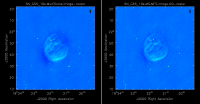
This is the fastest of the imaging techniques described here, but it's easy to see that there are artifacts in the resulting image. For example, use the {{viewer}} to explore the point sources near the edge of the field by zooming in on them. Some have prominent arcs, as well as spots in a six-pointed pattern surrounding them. Note that you may need to play with the brightness/contrast of the image to see more detail | This is the fastest of the imaging techniques described here, but it's easy to see that there are artifacts in the resulting image. For example, use the {{viewer}} to explore the point sources near the edge of the field by zooming in on them. Some have prominent arcs, as well as spots in a six-pointed pattern surrounding them. Note that you may need to play with the brightness/contrast of the image to see more detail, or change the color map under data display options. | ||
Next we will explore some more advanced imaging techniques to mitigate these artifacts. | |||
=== Multi-Scale, Wide-Field Clean (w-projection) === | |||
[[Image:SN_G55_MS_vs_MSwProj.png|200px|thumb|right|MS artifacts (left) vs. MS and w-projection artifacts (right)]] | |||
The next {{clean}} algorithm we will employ is w-projection, which is a wide-field imaging technique that takes into account the non-coplanarity of the baselines as a function of distance from the phase center. For wide-field imaging, the sky curvature and non-coplanar baselines results in a non-zero w-term. The w-term introduced by the sky and array curvature introduces a phase term that will limit the dynamic range of the resulting image. Applying 2-D imaging to such data will result in artifacts around sources away from the phase center, as we saw in running MS-CLEAN. Note that this affects mostly the lower frequency bands, especially for the more extended configurations, due to the field of view decreasing with higher frequencies. | |||
The w-term can be corrected by faceting (describe the sky curvature by many smaller planes) in either the image or uv-plane, or by employing w-projection. A combination of the two can also be employed within {{clean}} by setting the parameter gridmode='widefield'. If w-projection is employed, it will be done for each facet. Note that w-projections is an order of magnitude faster than the faceting algorithm, but will require more memory. | |||
[[Image:Faceting.png|200px|thumb|right| Faceting when using widefield gridmode, which can be used in conjunction with w-projection. ]] | |||
For more details on imaging and deconvolution, you can refer to the Astronomical Society of the Pacific Conference Series book entitled [http://www.aspbooks.org/a/volumes/table_of_contents/?book_id=292 Synthesis Imaging in Radio Astronomy II]. The chapters on [http://www.aspbooks.org/a/volumes/article_details/?paper_id=17942 Deconvolution] and [http://www.aspbooks.org/a/volumes/article_details/?paper_id=17953 Imaging with Non-Coplanar Arrays] may prove helpful. Also, a brief intro to the different clean algorithms can be found [http://www.aoc.nrao.edu/~rurvashi/ImagingAlgorithmsInCasa/node2.html#SECTION00223000000000000000 here]. For more details on W-Projection, as well as the algorithm itself, see [http://adsabs.harvard.edu/abs/2008ISTSP...2..647C "The Noncoplanar Baselines Effect in Radio Interferometry: The W-Projection Algorithm"]. | |||
<source lang="python"> | <source lang="python"> | ||
# In CASA | # In CASA | ||
clean(vis=' | clean(vis='SNR_G55_10s.calib.ms', imagename='SNR_G55_10s.ms.wProj', | ||
gridmode='widefield', imsize=1280, cell='8arcsec', | gridmode='widefield', imsize=1280, cell='8arcsec', | ||
wprojplanes=128, multiscale=[0,6,10,30,60], | wprojplanes=128, multiscale=[0,6,10,30,60], | ||
| Line 377: | Line 356: | ||
stokes='I', threshold='0.1mJy', usescratch=F, imagermode='csclean') | stokes='I', threshold='0.1mJy', usescratch=F, imagermode='csclean') | ||
viewer(' | viewer('SNR_G55_10s.ms.wProj.image') | ||
</source> | </source> | ||
* gridmode='widefield': Use the W-Projection algorithm. | * gridmode='widefield': Use the W-Projection algorithm. | ||
| Line 386: | Line 363: | ||
* wprojplanes=128: The number of W-Projection planes to use for deconvolution; 128 is the minimum recommended number. | * wprojplanes=128: The number of W-Projection planes to use for deconvolution; 128 is the minimum recommended number. | ||
This will take slightly longer than the previous imaging round; however, the resulting image has noticeably fewer artifacts. In particular, compare the same outlier source in the W-Projected image with the Multi-Scale-only image: note that the swept-back arcs have disappeared. There are still some obvious imaging artifacts remaining, though. | This will take slightly longer than the previous imaging round; however, the resulting image has noticeably fewer artifacts. In particular, compare the same outlier source in the Multi-Scale W-Projected image with the Multi-Scale-only image: note that the swept-back arcs have disappeared. There are still some obvious imaging artifacts remaining, though. | ||
=== Multi-Scale, Multi-Frequency Synthesis === | === Multi-Scale, Multi-Frequency Synthesis === | ||
Another consequence of simultaneously imaging the wide fractional bandwidths available with the EVLA is that the primary beam has substantial frequency-dependent variation over the observing band. If this is not accounted for, it will lead to imaging artifacts and compromise the achievable image rms. | [[Image:SN_G55_MS_vs_MSMFS.png|200px|thumb|right|MS artifacts (left) vs MS-MFS artifacts (right) near SNR, with nterms=2]] | ||
[[Image:SN_G55_MS.MFS.wProj.alpha.png|200px|thumb|right|Spectral Index image]] | |||
Another consequence of simultaneously imaging the wide fractional bandwidths available with the EVLA is that the primary beam has substantial frequency-dependent variation over the observing band. If this is not accounted for, it will lead to imaging artifacts and compromise the achievable image rms. | |||
If sources which are being imaged have intrinsically flat spectra, this will not be a problem. However, most astronomical objects are not flat-spectrum sources, and without any estimation of the intrinsic spectral properties, the fact that the primary beam is twice as large at 2 than at 1 GHz will have substantial consequences. | If sources which are being imaged have intrinsically flat spectra, this will not be a problem. However, most astronomical objects are not flat-spectrum sources, and without any estimation of the intrinsic spectral properties, the fact that the primary beam is twice as large at 2 than at 1 GHz will have substantial consequences. | ||
| Line 398: | Line 378: | ||
<source lang="python"> | <source lang="python"> | ||
# In CASA | # In CASA | ||
clean(vis=' | clean(vis='SNR_G55_10s.calib.ms', imagename='SNR_G55_10s.ms.MFS', | ||
imsize=1280, cell='8arcsec', mode='mfs', nterms=2, | imsize=1280, cell='8arcsec', mode='mfs', nterms=2, | ||
multiscale=[0,6,10,30,60], | multiscale=[0,6,10,30,60], | ||
| Line 404: | Line 384: | ||
stokes='I', threshold='0.1mJy', usescratch=F, imagermode='csclean') | stokes='I', threshold='0.1mJy', usescratch=F, imagermode='csclean') | ||
viewer(' | viewer('SNR_G55_10s.ms.MFS.image.tt0') | ||
viewer(' | viewer('SNR_G55_10s.ms.MFS.image.alpha') | ||
</source> | </source> | ||
* nterms=2:the number of Taylor terms to be used to model the frequency dependence of the sky emission. Note that the speed of the algorithm will depend on the value used here (more terms will be slower); of course, the image fidelity will improve with a larger number of terms (assuming the sources are sufficiently bright to be modeled more completely). | * nterms=2:the number of Taylor terms to be used to model the frequency dependence of the sky emission. Note that the speed of the algorithm will depend on the value used here (more terms will be slower); of course, the image fidelity will improve with a larger number of terms (assuming the sources are sufficiently bright to be modeled more completely). | ||
| Line 415: | Line 393: | ||
This will take much longer than the two previous methods, so it would probably be a good time to have coffee or chat about EVLA data reduction with your neighbor at this point. | This will take much longer than the two previous methods, so it would probably be a good time to have coffee or chat about EVLA data reduction with your neighbor at this point. | ||
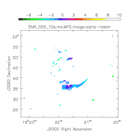
When clean is done <imagename>.image.tt0 will contain a total intensity image; <imagename>.image.alpha will contain an image of the spectral index in regions where there is sufficient signal-to-noise. | When clean is done <imagename>.image.tt0 will contain a total intensity image, where tt0 is a suffix to indicate the Taylor term; <imagename>.image.alpha will contain an image of the spectral index in regions where there is sufficient signal-to-noise. Having this spectral index image can help convey information about the emission mechanism involved within the supernova remnant. It can also give information on the optical depth of the source. I've included a color widget on the top of the plot to give an idea of the spectral index variation. | ||
For more information on the multi-frequency synthesis mode and its outputs, see section 5.2.5.1 in the [http://casa.nrao.edu/Doc/Cookbook/casa_cookbook.pdf CASA cookbook]. | |||
Inspect the brighter point sources in the field near the supernova remnant. You will notice that some of the artifacts which had been symmetric around the sources themselves are now gone; however, since we did not use W-Projection this time, there are still strong features related to the non-coplanar baseline effects still apparent for sources further away. | |||
First, we will image the autoflagged data. | === Multi-Scale, Multi-Frequency, Widefield Clean === | ||
Finally, we will combine the W-Projection and MS-MFS algorithms to simultaneously account for both of the effects. Be forewarned -- these imaging runs will take a while, and it's best to start them running and then move on to other things. | |||
First, we will image the autoflagged data. Using the same parameters for the individual-algorithm images above, but combined into a single {{clean}} run, we have: | |||
[[Image:SN_G55.MS.MFS.wProj.png|200px|thumb|right| The combination of W-Projection and MS-MFS with nterms=2]] | |||
<source lang="python"> | <source lang="python"> | ||
# In CASA | # In CASA | ||
clean(vis=' | clean(vis='SNR_G55_10s.calib.ms', imagename='SNR_G55_10s.ms.MFS.wProj', | ||
gridmode='widefield', imsize=1280, cell='8arcsec', mode='mfs', | gridmode='widefield', imsize=1280, cell='8arcsec', mode='mfs', | ||
nterms=2, wprojplanes=128, multiscale=[0,6,10,30,60], | nterms=2, wprojplanes=128, multiscale=[0,6,10,30,60], | ||
interactive=False, niter=1000, weighting='briggs', | interactive=False, niter=1000, weighting='briggs', | ||
stokes='I', threshold='0.1mJy', usescratch=F, imagermode='csclean') | stokes='I', threshold='0.1mJy', usescratch=F, imagermode='csclean') | ||
viewer(' | |||
viewer(' | viewer('SNR_G55_10s.ms.MFS.wProj.image.tt0') | ||
viewer('SNR_G55_10s.ms.MFS.wProj.image.alpha') | |||
</source> | </source> | ||
Again, looking at the same outlier source, we can see that the major sources of error have been removed, although there are still some residual artifacts. One possible source of error is the time-dependent variation of the primary beam; another is the fact that we have only used nterms=2, which may not be sufficient to model the spectra of some of the point sources. | Again, looking at the same outlier source, we can see that the major sources of error have been removed, although there are still some residual artifacts. One possible source of error is the time-dependent variation of the primary beam; another is the fact that we have only used nterms=2, which may not be sufficient to model the spectra of some of the point sources. | ||
Ultimately, it isn't too surprising that there was still some RFI present in our auto-flagged data, since we were able to see this with {{plotms}}. It's also possible that the auto-flagging overflagged some portions of the data, also leading to a reduction in the achievable image rms. | |||
=== Imaging Weighting === | |||
When imaging data, a map is created associating the visibilities with the image. This sampling function is modified by the weight introduced during deconvolution <math>S(u,v) \to S(u,v)W(u,v)</math>. The convolution map, is the weights by which each visiblity is multiplied by before gridding is undertaken. Due to the fact that each VLA antenna performs slightly differently, different weights should be applied to each antenna. The weight column in the data table reflects how much weight each corrected data sample should receive. | |||
The following forms of weighting can be used within the {{clean}} task. Each one has their own benefits and drawbacks. | |||
1. | |||
=== Imaging with tclean === | |||
The tclean task will eventually be replacing clean as the default when imaging, so it would be a good idea to familiarize ourselves with the parameters, which differ from clean. Let us now create the same MS-MFS, w-projection image, via tclean: | |||
<source lang="python"> | <source lang="python"> | ||
# In CASA | # In CASA | ||
tclean(vis='SNR_G55_10s.calib.ms', imagename='SNR_G55_10s.tclean.MS.MFS.wProj', imsize=1280, | |||
cell='8arcsec', specmode='mfs', gridder='wproject', wprojplanes=256, | |||
deconvolver='multiscale', scales=[0,6,10,30,60], interactive=False, niter=1000, | |||
weighting='briggs', stokes='I', threshold='0.1mJy', nterms=2) | |||
</source> | </source> | ||
We can now specify w-projection within the gridder parameter (gridmode in clean), and mfs within the specmode parameter (mode in clean). In addition, you will notice the tclean process runs faster than clean. tclean also has a parallel parameter, which will run major cycles in parallel. This option is set to False by default, as it requires MPI (Message Passing Interface) to be enabled on your system for tclean to run. See chapter 10 in the CASA Cookbook. | |||
[[Main Page | ↵ '''CASAguides''']] | [[Main Page | ↵ '''CASAguides''']] | ||
Revision as of 18:59, 29 March 2016
- Topical guide, part 2 of 2
- This CASA guide is designed for CASA 4.5.2
Overview
This CASA guide will cover data calibration and advanced imaging. Such topics include MS (Multi Scale) on regular images, MS-MFS (Multi Scale-Multi Frequency Scale), W-Projection, Wide Field Mode, outlier fields, spectral indices, and interactive mode.
JVLA - Importing and Initial Flagging in CASA:Part 1 of the guide covered the importing of the dataset, time-averaging, and data flagging, including shadow, zero-clipping, tfcrop, rflag, quacking, and online flagging.
We will be utilizing data taken with the Karl G. Jansky, Very Large Array, of a supernova remnant G055.7+3.4.. The data were taken on August 23, 2010, in the first D-configuration for which the new wide-band capabilities of the WIDAR (Wideband Interferometric Digital ARchitecture) correlator were available. The 8-hour-long observation includes all available 1 GHz of bandwidth in L-band, from 1-2 GHz in frequency.
Obtaining the Data
We will be utilizing the time-averaged and flagged data from part 1. If you'd like to skip the first part of the tutorial and delve into part 2, you can acquire the measurement set for this tutorial here.
Start and confirm your version of CASA
Start CASA by typing casa on a terminal command line. If you have not used CASA before, some helpful tips are available on the Getting Started in CASA page.
This guide has been written for CASA release 4.5.2. Please confirm your version before proceeding by checking the message in the command line interface window or the CASA logger after startup.
Calibrating Data
Now that we are satisfied with the RFI excision, we will move on to the calibration stage.
Flux Density Scale
Since we will be using 3C147 as the source of the absolute flux scale for this observation, we must first run setjy to set the appropriate model amplitudes for this source.
If the flux calibrator is spatially resolved, it is necessary to include a model image as well. Although 3C147 is not resolved at L-band in D configuration, we include the model image here for completeness.
First, we use the listmodimages parameter to find the model image path:
# In CASA
setjy(vis='SNR_G55_10s.ms', listmodels=True)
This lists any images in the current working directory as well as images in CASA's repository. In this second list, we see that there is "3C147_L.im", which is appropriate for our flux calibrator and band, and that it is in the directory "/home/casa/packages/RHEL6/release/casa-release-4.4.0/data/nrao/VLA/CalModels ". We can optionally give the full path of the model image, but setjy should now be able to locate it by name alone:
# In CASA
setjy(vis='SNR_G55_10s.ms', field='0542*', scalebychan=True, model='3C147_L.im')
- scalebychan=True: scales the model flux density value for each channel.
Note: The task setjy uses the Perley-Butler 2010 standard by default. Periodically, the flux density scale at the VLA is revised, updated, or expanded. The most recent standard is Perley-Butler 2013, and can be used by explicitly setting standard='Perley-Butler 2013' in the task. See help setjy for more details.
Ionospheric TEC Corrections
Low frequency observations (4 through S Bands) are affected by the ionosphere conditions. A delay can be introduced into the signal path, which is proportional to the Total Electron Content (TEC) along the line of sight, and is inversely proportional to the square of the frequency. We can apply a correction by utilizing GPS measurements taken at two different frequencies from the IGS (International GPS Services) website. We will utilize the gencal task with paramter caltype set to 'tecim'. This should generate a plot of TEC vs Time for the VLA site, for the day of the observation.
# In CASA
tec_image, tec_rms_image = tec_maps.create(vis='SNR_G55_10s.ms',doplot=True)

gencal(vis='SNR_G55_10s.ms',caltable='SNR_G55_10s.tecim',caltype='tecim',infile=tec_image)
The resulting images can be inspected with the CASA viewer task. As we can see, there was a lot of ionospheric activity on this particular day, therefore applying this correction can result in a better image quality for low-band observing.
Delay and Bandpass Calibration
We will follow a similar procedure as the one outlined in part 1, when we created the preliminary bandpass calibration table SN_G55_10s.initPh. This time, we will use the actual designated bandpass calibration source 0542+498=3C147. Although the phase calibration source used previously (J1925+2106) has the advantage of having been observed throughout the run, it has an unknown spectrum which could introduce amplitude slopes to each spectral window. In addition, we will calibrate the residual antenna-based delays (for further information on this topic, please see this tutorial: [[1]].)
As before, we first generate a phase-only gain calibration table that will be used to help smooth-out the phases before running bandpass itself:
# In CASA
gaincal(vis='SNR_G55_10s.ms', field = '2',
        caltable='SNR_G55_10s.initPh.2',
        spw='*:45~49', solint='int', refant='ea24',
        minblperant=3, minsnr=3.0, calmode='p',
        gaintable=['SNR_G55_10s.pos', 'SNR_G55_10s.tecim'])
Again, you will notice a few messages that read "Insufficient unflagged antennas to proceed with this solve."
We can now solve for the residual antenna-based delays that can be seen in plots of the phase vs. frequency for the calibrator sources in plotms. This uses the gaintype='K' option in gaincal. Note that this currently does not do a "global fringe-fitting" solution for delays, but instead does a baseline-based delay solution to all baselines to the refant, treating these as antenna-based delays. In most cases with high-enough S/N to get baseline-based delay solutions this will suffice. We use our bright bandpass calibrator, 3C147, to calibrate the delays:
# In CASA
gaincal(vis='SNR_G55_10s.ms', field='2',
        caltable='SNR_G55_10s.K0',
        solint='inf', refant='ea24',
        gaintype='K', combine='scan', minsnr=3,
        gaintable=['SNR_G55_10s.pos', 'SNR_G55_10s.tecim', 'SNR_G55_10s.initPh.2'])
We pre-apply our initial phase table, and produce a new K-type caltable for input to bandpass calibration. We can plot the delays, in nanoseconds, as a function of antenna index (you will get one for each sub-band and polarization):
# In CASA
plotcal(caltable='SNR_G55_10s.K0', xaxis='antenna', yaxis='delay')
The delays range from around -3 to 5 nanoseconds, which is good. Anything over 10ns would be cause for concern.
Now let's solve for the bandpass using the previous tables:
# In CASA
bandpass(vis='SNR_G55_10s.ms', caltable='SNR_G55_10s.bPass',
         field='2', solint='inf', combine='scan',
	 refant='ea24', minblperant=3, minsnr=10.0,
         gaintable=['SNR_G55_10s.pos', 'SNR_G55_10s.tecim', 'SNR_G55_10s.initPh.2','SNR_G55_10s.K0'],
         interp=['', 'nearest', 'nearest'], solnorm=False)
- solint='inf', combine='scan': again, the solution interval of 'inf' will automatically break-up the data by scans; this requests that the solution intervals be combined over scans, so that we will get one solution per antenna. Note that you must set solnorm=False here or later on you will find some offsets between spws due to the way in which amplitude scaling adjusts weights internally during solving.
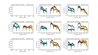
Note that since we have flagged-out the vast majority of the RFI-affected data, there are many fewer failed solutions. Again, we can plot the calculated bandpasses to check that they look reasonable:
# In CASA
plotcal(caltable='SNR_G55_10s.bPass', xaxis='freq', yaxis='amp',
        iteration='antenna', subplot=331)
#
plotcal(caltable='SNR_G55_10s.bPass', xaxis='freq', yaxis='phase',
        iteration='antenna', subplot=331)
Don't let the apparently odd-looking phases for ea24 fool you -- check the scale! Remember, this is our reference antenna.
Gain calibration
Next, we will calculate the per-antenna gain solutions. We will now use the intent parameter. Since this is low-frequency data, we do not expect substantial variations over short timescales, so we calculate one solution per scan (using solint='inf'):
# In CASA
gaincal(vis='SNR_G55_10s.ms', caltable='SNR_G55_10s.phaseAmp',
        intent='*PHASE*,*AMPLI*', solint='inf', refant='ea24', minblperant=3,
        minsnr=10.0, gaintable=['SNR_G55_10s.pos', 'SNR_G55_10s.tecim', 'SNR_G55_10s.K0','SNR_G55_10s.bPass'])
- solint='inf': we request one solution per scan.
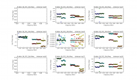
Plot these solutions as a function of amplitude and phase versus time for the phase calibrator (field 0), iterating over each antenna:
# In CASA
plotcal(caltable='SNR_G55_10s.phaseAmp', xaxis='time', yaxis='amp',
        field = '0', iteration='antenna')

plotcal(caltable='SNR_G55_10s.phaseAmp', xaxis='time', yaxis='phase',
        field = '0', plotsymbol='-', iteration='antenna')
Flux Scaling the Gain Solutions
Now that we have a complete set of gain solutions, we must scale the phase calibrator's absolute flux correctly, using 3C147 as our reference source. To do this, we run fluxscale on the gain table we just created, which will write a new, flux-corrected gain table (SNR_G55_10s.phaseAmp.fScale):
# In CASA
myFlux = fluxscale(vis='SNR_G55_10s.ms', caltable='SNR_G55_10s.phaseAmp',
         fluxtable='SNR_G55_10s.phaseAmp.fScale', reference='2', incremental=False)
Note that the myFlux Python dictionary will contain information about the scaled fluxes and fitted spectrum. The logger will display information about the flux density it has deduced for J1925+2106:
2016-03-16 21:16:00 INFO fluxscale	 Found reference field(s): 0542+498=3C147
2016-03-16 21:16:00 INFO fluxscale	 Found transfer field(s):  J1925+2106
2016-03-16 21:16:01 INFO fluxscale	 Flux density for J1925+2106 in SpW=0 (freq=1.319e+09 Hz) is: 1.50509 +/- 0.0283309 (SNR = 53.1254, N = 40)
2016-03-16 21:16:01 INFO fluxscale	 Flux density for J1925+2106 in SpW=1 (freq=1.447e+09 Hz) is: 1.56106 +/- 0.0252717 (SNR = 61.7711, N = 40)
2016-03-16 21:16:01 INFO fluxscale	 Flux density for J1925+2106 in SpW=2 (freq=1.711e+09 Hz) is: 1.71527 +/- 0.0249139 (SNR = 68.8477, N = 40)
2016-03-16 21:16:01 INFO fluxscale	 Flux density for J1925+2106 in SpW=3 (freq=1.839e+09 Hz) is: 1.7623  +/- 0.0265479 (SNR = 66.382,  N = 40)
2016-03-16 21:16:01 INFO fluxscale	 Fitted spectrum for J1925+2106 with fitorder=1: Flux density = 1.63244 +/- 0.00551612 (freq=1.56544 GHz) spidx=0.495241 +/- 0.0264202
The flux density listed in the VLA Calibrator Manual for J1925+2106 (known then as J1925+211 for J2000 epoch) is around the same magnitude at L-Band:
1925+211   J2000  A 19h25m59.605370s  21d06'26.162180"  Aug01
1923+210   B1950  A 19h23m49.792400s  21d00'23.305000"
-----------------------------------------------------
BAND        A B C D    FLUX(Jy)    UVMIN(kL)  UVMAX(kL)
=====================================================
 20cm    L  P S S S       1.30                       visplot
  6cm    C  P P S S       1.5
3.7cm    X  P P P P       1.00                       visplot
  2cm    U  P P P P       1.8
1.3cm    K  S S S S       0.90                       visplot
0.7cm    Q  S S S S       1.0
This is a good indication that our calibration up to this point is reasonable. We will now apply these calibration tables to our data, and begin our imaging.
Applying calibration
Finally, we must apply the calibration to our data. To do this, we run applycal in two stages: the first is to self-calibrate our calibration sources; the second, to apply calibration to the supernova remnant. These must be done separately, since we want to use "nearest" interpolation for the self-calibration and "linear" (this is the default, so we can omit requesting the interpolation) for the application to the science target:
# In CASA
applycal(vis='SNR_G55_10s.ms', intent='*PHASE*,*AMPLI*',
         gaintable=['SNR_G55_10s.pos', 'SNR_G55_10s.tecim', 'SNR_G55_10s.K0',
                    'SNR_G55_10s.bPass', 'SNR_G55_10s.phaseAmp.fScale'],
         calwt=False, interp=['','nearest','nearest','nearest'])

applycal(vis='SNR_G55_10s.ms', intent='*TARGET*',
         gaintable=['SNR_G55_10s.pos', 'SNR_G55_10s.tecim', 'SNR_G55_10s.K0',
                    'SNR_G55_10s.bPass', 'SNR_G55_10s.phaseAmp.fScale'], calwt=False)
Plotting calibrated data
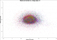
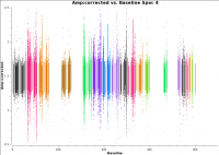
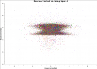
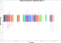
To check that everything has truly proceeded as well as we would like, this is a good time to look at the calibrated data in plotms. A very useful way to check the quality of the calibration, is to plot the corrected real vs. imaginary portions of the visibilities of our calibrators.
For a point source at the phase center, the plot should look like scatter around zero for the imaginary axis (zero phase), and scatter around the flux density value (amplitude) of the source, in the real axis. The corrected amplitude vs. baseline, which should be a flat line of points for a point source, will reveal any lingering antenna-based problems. For a resolved source, it may be more instructive to plot corrected amplitude vs. UV-distance.
# In CASA
plotms(vis='SNR_G55_10s.ms', field='0', xaxis='imag', yaxis='real',
       xdatacolumn='corrected', ydatacolumn='corrected', coloraxis='antenna1',
       avgchannel='10', avgtime='30', correlation='RR,LL', iteraxis='spw',
       plotrange=[-1.5,1.5,0,2.8])
#
plotms(vis='SNR_G55_10s.ms', field='0', xaxis='baseline', yaxis='amp',
       xdatacolumn='corrected', ydatacolumn='corrected', coloraxis='antenna1',
       avgchannel='10', avgtime='30', correlation='RR,LL', iteraxis='spw',
       plotrange=[0,450,0.5,2.5])
#
plotms(vis='SNR_G55_10s.ms', field='2', xaxis='imag', yaxis='real',
       xdatacolumn='corrected', ydatacolumn='corrected', coloraxis='antenna1',
       avgchannel='10', avgtime='30', correlation='RR,LL', iteraxis='spw',
       plotrange=[-5,5,18,28])
#
plotms(vis='SNR_G55_10s.ms', field='2', xaxis='baseline', yaxis='amp',
       xdatacolumn='corrected', ydatacolumn='corrected', coloraxis='antenna1',
       avgchannel='10', avgtime='30', correlation='RR,LL', iteraxis='spw',
       plotrange=[0,450,18,28])
Splitting out data for G55.7+3.4
Now that we are satisfied with the calibration, we will create a new MS which contains only the corrected data for G55.7+3.4 using the task split2. The split task is used to make a new data set that is a subset of an existing data set. The Split2 task provides the functionality of split, but is based on the mstransform framework underneath, which is more versatile. For more on split2, see the CASA Cookbook, section 4.7.4.1. Starting with CASA version 4.6, the split2 task will be renamed split, and replace the current split task.
Splitting out just the target we want to image will substantially reduce the size of the MS, and will speed up the imaging process. We can also drop the polarization products since they have not been calibrated and will not be used for imaging.
# In CASA
split2(vis='SNR_G55_10s.ms', field='1', keepflags=False,
      outputvis='SNR_G55_10s.calib.ms', datacolumn='corrected',
      correlation = 'RR,LL')
Imaging
The primary beam of the VLA antennas can be taken to be a Gaussian with FWHM equal to [math]\displaystyle{ 90*\lambda_{cm} }[/math] or [math]\displaystyle{ 45/ \nu_{GHz} }[/math]. Taking our observed frequency to be the middle of the band, 1.5GHz, our primary beam will be around 30 arcmin. Note that if your science goal is to image a source, or field of view that is significantly larger than the FWHM of the VLA primary beam, then creating a mosaic from a number of pointings would be best. For a tutorial on mosaicing, see the 3C391 tutorial.
Since our observation was taken in D-configuration, we can check the Observational Status Summary's section on VLA resolution to find that the synthesized beam will be around 46 arcsec. We want to oversample the synthesized beam by a factor of around five, so we will use a cell size of 8 arcsec.
Since this field contains bright point sources significantly outside the primary beam, we will create images that are 170 arcminutes on a side, or almost 6x the size of the primary beam. This is ideal for showcasing both the problems inherent in such wide-band, wide-field imaging, as well as some of the solutions currently available in CASA to deal with these issues.
First, it's worth considering why we are even interested in sources which are far outside the primary beam. This is mainly due to the fact that the EVLA, with its wide bandwidth capabilities, is quite sensitive even far from phase center -- for example, at our observing frequencies in L-band, the primary beam gain is as much as 10% around 1 degree away. That means that any imaging errors for these far-away sources will have a significant impact on the image rms at phase center. The error due to a source at distance R can be parametrized as:
[math]\displaystyle{ \Delta(S) = S(R) \times PB(R) \times PSF(R) }[/math]
So, for R = 1 degree, source flux S(R) = 1 Jy, [math]\displaystyle{ \Delta(S) }[/math] = 1 mJy − 100 [math]\displaystyle{ {\mu} }[/math]Jy. Clearly, this will be a source of significant error.
Multi-Scale Clean
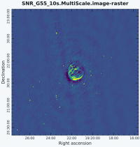
Since G55.7+3.4 is an extended source with many spatial scales, the most basic (yet still reasonable) imaging procedure is to use clean with multiple scales. MS-CLEAN is an extension of the classical CLEAN algorithm for handling extended sources. It works by assuming the sky is composed of emission at different spatial scales and works on them simultaneously.
It can also be possible to utilize tclean, (t for test) which is a refactored version of clean, with a better interface, and provides more possible combinations of algorithms. It also allows for process computing parallelization of the imaging and deconvolution. Eventually, tclean will replace the current clean task, but for now, we will stick with the original clean, as tclean is merely experimental at the moment.
As is suggested, we will use a set of scales (which are expressed in units of the requested pixel, or cell, size) which are representative of the scales that are present in the data, including a zero-scale for point sources.
Note that interrupting clean by Ctrl+C may corrupt your visibilities -- you may be better off choosing to let clean finish. We are currently implementing a command that will nicely exit to prevent this from happening, but for the moment try to avoid Ctrl+C.
# In CASA
clean(vis='SNR_G55_10s.calib.ms', imagename='SNR_G55_10s.MultiScale',
      imsize=1280, cell='8arcsec', multiscale=[0,6,10,30,60], smallscale=0.9,
      interactive=False, niter=1000,  pbcor=True, weighting='briggs', uvtaper='
      stokes='I', threshold='0.1mJy', usescratch=F, imagermode='csclean')

clean(vis='SNR_G55_10s.calib.ms', imagename='SNR_G55_10s.MultiScale',
      imsize=1280, cell='8arcsec', multiscale=[0,6,10,30,60],
      interactive=False, niter=1000,  weighting='briggs',
      stokes='I', threshold='0.1mJy', usescratch=F, imagermode='csclean')

viewer('SN_G55_10s.MultiScale.image')
- imagename='SN_G55_10s.MultiScale': the root filename used for the various clean outputs. These include the final image (<imagename>.image), the relative sky sensitivity over the field (<imagename>.flux), the point-spread function (also known as the dirty beam; <imagename>.psf), the clean components (<imagename>.model), and the residual image (<imagename>.residual).
- imsize=1280: the image size in number of pixels. Note that entering a single value results in a square image with sides of this value.
- cell='8arcsec': the size of one pixel; again, entering a single value will result in a square pixel size.
- multiscale=[0,6,10,30,60]: a set of scales on which to clean. A good rule of thumb when using multiscale is [0, 2xbeam, 5xbeam] (where beam is the synthesized beam) and larger scales up to the maximum scale the interferometer can image. Since these are in units of the pixel size, our chosen values will be multiplied by the requested cell size. Thus, we are requesting scales of 0 (a point source), 48, 80, 240, and 480 arcseconds. Note that 16 arcminutes (960 arcseconds) roughly corresponds to the size of G55.7+3.4.
- smallscale=0.9: This parameter helps with faint extended structure, by balancing the weight given to smaller structures which tend to be brighter, but have less flux density. Increasing this value gives more weight to smaller scales. A value of 1.0 weighs the largest scale to zero, and a value of less than 0.2 weighs all scales nearly equally. The default value is 0.6.
- interactive=False: we will let clean use the entire field for placing model components. Alternatively, you could try using interactive=True, and create regions to constrain where components will be placed. However, this is a very complex field, and creating a region for every bit of diffuse emission as well as each point source can quickly become tedious. For a tutorial that covers more of an interactive clean, please see IRC+10216 tutorial.
- niter=1000: this controls the number of iterations clean will do in the minor cycle.
- pbcor=True: We can correct for the relative sky sensitivity while running clean. This will help in creating a near circularly symmetric beam, which may be better able to image extended sources, over long observations. setting this to true, forces the raw image to be rescaled by dividing by the noise and primary beam correction image (<imagename>.flux). Note that this can also be done via the immath task if pbcor=False.
- weighting='briggs': use Briggs weighting with a robustness parameter of 0 (halfway between uniform and natural weighting).
- usescratch=F: do not write the model visibilities to the model data column (only needed for self-calibration)
- imagermode='csclean': use the Cotton-Schwab clean algorithm
- stokes='I': since we have not done any polarization calibration, we only create a total-intensity image.
- threshold='0.1mJy': threshold at which the cleaning process will halt; i.e. no clean components with a flux less than this value will be created. This is meant to avoid cleaning what is actually noise (and creating an image with an artificially low rms). It is advisable to set this equal to the expected rms, which can be estimated using the EVLA exposure calculator. However, in our case, this is a bit difficult to do, since we have lost a hard-to-estimate amount of bandwidth due to flagging, and there is also some residual RFI present. Therefore, we choose 0.1 mJy as a relatively conservative limit.
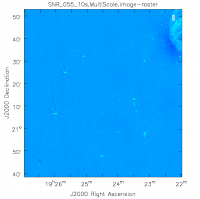
This is the fastest of the imaging techniques described here, but it's easy to see that there are artifacts in the resulting image. For example, use the viewer to explore the point sources near the edge of the field by zooming in on them. Some have prominent arcs, as well as spots in a six-pointed pattern surrounding them. Note that you may need to play with the brightness/contrast of the image to see more detail, or change the color map under data display options.
Next we will explore some more advanced imaging techniques to mitigate these artifacts.
Multi-Scale, Wide-Field Clean (w-projection)
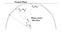
The next clean algorithm we will employ is w-projection, which is a wide-field imaging technique that takes into account the non-coplanarity of the baselines as a function of distance from the phase center. For wide-field imaging, the sky curvature and non-coplanar baselines results in a non-zero w-term. The w-term introduced by the sky and array curvature introduces a phase term that will limit the dynamic range of the resulting image. Applying 2-D imaging to such data will result in artifacts around sources away from the phase center, as we saw in running MS-CLEAN. Note that this affects mostly the lower frequency bands, especially for the more extended configurations, due to the field of view decreasing with higher frequencies.
The w-term can be corrected by faceting (describe the sky curvature by many smaller planes) in either the image or uv-plane, or by employing w-projection. A combination of the two can also be employed within clean by setting the parameter gridmode='widefield'. If w-projection is employed, it will be done for each facet. Note that w-projections is an order of magnitude faster than the faceting algorithm, but will require more memory.
For more details on imaging and deconvolution, you can refer to the Astronomical Society of the Pacific Conference Series book entitled Synthesis Imaging in Radio Astronomy II. The chapters on Deconvolution and Imaging with Non-Coplanar Arrays may prove helpful. Also, a brief intro to the different clean algorithms can be found here. For more details on W-Projection, as well as the algorithm itself, see "The Noncoplanar Baselines Effect in Radio Interferometry: The W-Projection Algorithm".
# In CASA
clean(vis='SNR_G55_10s.calib.ms', imagename='SNR_G55_10s.ms.wProj',
      gridmode='widefield', imsize=1280, cell='8arcsec',
      wprojplanes=128, multiscale=[0,6,10,30,60],
      interactive=False, niter=1000,  weighting='briggs',
      stokes='I', threshold='0.1mJy', usescratch=F, imagermode='csclean')

viewer('SNR_G55_10s.ms.wProj.image')
- gridmode='widefield': Use the W-Projection algorithm.
- wprojplanes=128: The number of W-Projection planes to use for deconvolution; 128 is the minimum recommended number.
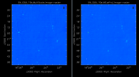
This will take slightly longer than the previous imaging round; however, the resulting image has noticeably fewer artifacts. In particular, compare the same outlier source in the Multi-Scale W-Projected image with the Multi-Scale-only image: note that the swept-back arcs have disappeared. There are still some obvious imaging artifacts remaining, though.
Multi-Scale, Multi-Frequency Synthesis
Another consequence of simultaneously imaging the wide fractional bandwidths available with the EVLA is that the primary beam has substantial frequency-dependent variation over the observing band. If this is not accounted for, it will lead to imaging artifacts and compromise the achievable image rms.
If sources which are being imaged have intrinsically flat spectra, this will not be a problem. However, most astronomical objects are not flat-spectrum sources, and without any estimation of the intrinsic spectral properties, the fact that the primary beam is twice as large at 2 than at 1 GHz will have substantial consequences.
The Multi-Scale Multi-Frequency-Synthesis (MS-MFS) algorithm provides the ability to simultaneously image and fit for the intrinsic source spectrum. The spectrum is approximated using a polynomial in frequency, with the degree of the polynomial as a user-controlled parameter. A least-squares approach is used, along with the standard clean-type iterations.
# In CASA
clean(vis='SNR_G55_10s.calib.ms', imagename='SNR_G55_10s.ms.MFS',
      imsize=1280, cell='8arcsec', mode='mfs', nterms=2,
      multiscale=[0,6,10,30,60],
      interactive=False, niter=1000,  weighting='briggs',
      stokes='I', threshold='0.1mJy', usescratch=F, imagermode='csclean')

viewer('SNR_G55_10s.ms.MFS.image.tt0')

viewer('SNR_G55_10s.ms.MFS.image.alpha')
- nterms=2:the number of Taylor terms to be used to model the frequency dependence of the sky emission. Note that the speed of the algorithm will depend on the value used here (more terms will be slower); of course, the image fidelity will improve with a larger number of terms (assuming the sources are sufficiently bright to be modeled more completely).
This will take much longer than the two previous methods, so it would probably be a good time to have coffee or chat about EVLA data reduction with your neighbor at this point.
When clean is done <imagename>.image.tt0 will contain a total intensity image, where tt0 is a suffix to indicate the Taylor term; <imagename>.image.alpha will contain an image of the spectral index in regions where there is sufficient signal-to-noise. Having this spectral index image can help convey information about the emission mechanism involved within the supernova remnant. It can also give information on the optical depth of the source. I've included a color widget on the top of the plot to give an idea of the spectral index variation.
For more information on the multi-frequency synthesis mode and its outputs, see section 5.2.5.1 in the CASA cookbook.
Inspect the brighter point sources in the field near the supernova remnant. You will notice that some of the artifacts which had been symmetric around the sources themselves are now gone; however, since we did not use W-Projection this time, there are still strong features related to the non-coplanar baseline effects still apparent for sources further away.
Multi-Scale, Multi-Frequency, Widefield Clean
Finally, we will combine the W-Projection and MS-MFS algorithms to simultaneously account for both of the effects. Be forewarned -- these imaging runs will take a while, and it's best to start them running and then move on to other things.
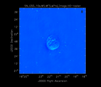
First, we will image the autoflagged data. Using the same parameters for the individual-algorithm images above, but combined into a single clean run, we have:
# In CASA
clean(vis='SNR_G55_10s.calib.ms', imagename='SNR_G55_10s.ms.MFS.wProj',
      gridmode='widefield', imsize=1280, cell='8arcsec', mode='mfs',
      nterms=2, wprojplanes=128, multiscale=[0,6,10,30,60],
      interactive=False, niter=1000,  weighting='briggs',
      stokes='I', threshold='0.1mJy', usescratch=F, imagermode='csclean')

viewer('SNR_G55_10s.ms.MFS.wProj.image.tt0')

viewer('SNR_G55_10s.ms.MFS.wProj.image.alpha')
Again, looking at the same outlier source, we can see that the major sources of error have been removed, although there are still some residual artifacts. One possible source of error is the time-dependent variation of the primary beam; another is the fact that we have only used nterms=2, which may not be sufficient to model the spectra of some of the point sources.
Ultimately, it isn't too surprising that there was still some RFI present in our auto-flagged data, since we were able to see this with plotms. It's also possible that the auto-flagging overflagged some portions of the data, also leading to a reduction in the achievable image rms.
Imaging Weighting
When imaging data, a map is created associating the visibilities with the image. This sampling function is modified by the weight introduced during deconvolution [math]\displaystyle{ S(u,v) \to S(u,v)W(u,v) }[/math]. The convolution map, is the weights by which each visiblity is multiplied by before gridding is undertaken. Due to the fact that each VLA antenna performs slightly differently, different weights should be applied to each antenna. The weight column in the data table reflects how much weight each corrected data sample should receive.
The following forms of weighting can be used within the clean task. Each one has their own benefits and drawbacks. 1.
Imaging with tclean
The tclean task will eventually be replacing clean as the default when imaging, so it would be a good idea to familiarize ourselves with the parameters, which differ from clean. Let us now create the same MS-MFS, w-projection image, via tclean:
# In CASA
tclean(vis='SNR_G55_10s.calib.ms', imagename='SNR_G55_10s.tclean.MS.MFS.wProj', imsize=1280,
      cell='8arcsec', specmode='mfs', gridder='wproject', wprojplanes=256,
      deconvolver='multiscale', scales=[0,6,10,30,60], interactive=False, niter=1000,
      weighting='briggs', stokes='I', threshold='0.1mJy', nterms=2)
We can now specify w-projection within the gridder parameter (gridmode in clean), and mfs within the specmode parameter (mode in clean). In addition, you will notice the tclean process runs faster than clean. tclean also has a parallel parameter, which will run major cycles in parallel. This option is set to False by default, as it requires MPI (Message Passing Interface) to be enabled on your system for tclean to run. See chapter 10 in the CASA Cookbook.
-- original: ??
--modifications: Lorant Sjouwerman (4.4.0, 2015/07/07)
--modifications: Jose Salcido (4.5.2, 2016/02/24)
Last checked on CASA Version 4.5.2
