IRAS16293 Band9 - Imaging for CASA 3.4: Difference between revisions
No edit summary |
No edit summary |
||
| Line 50: | Line 50: | ||
<source lang="python"> | <source lang="python"> | ||
# Make a plot of the mosaic pattern with field ids identified | |||
aU.plotMosaic(vis='IRAS16293_Band9.ms',sourceid='0', | aU.plotMosaic(vis='IRAS16293_Band9.ms',sourceid='0', | ||
doplot=True,figfile='mosaic_pattern.png') | doplot=True,figfile='mosaic_pattern.png') | ||
</source> | </source> | ||
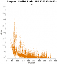
You might wander what of these pointings or fields have stronger line emission. You can know this by running the next command. We set spw='1', and you can check all the plots for all the fields by just hitting the arrow for "next". Also see Figure 2 for an example of the output. | |||
[[File:IRAS16293B9_uvamp_f2.png|200px|thumb|right|'''Fig. 2.''' UV-amp distribution for the field 2 in the mosaic.]] | |||
<source lang="python"> | |||
# See which mosaic fields have the brightest line emission | |||
plotms(vis='IRAS16293_Band9.ms', | |||
field='',xaxis='uvdist', yaxis='amp', | |||
spw='1', avgchannel='3840',coloraxis='field', | |||
iteraxis='field') | |||
</source> | |||
Revision as of 11:22, 23 May 2012
Overview
This section of the casa guide continues from the last step of the calibration one. If you completed the calibration section, then you already have the final calibrated dataset. If you just started to work on this IRAS16293 B9 data, you can download the fully calibrated dataset IRAS16293_Band9_CalibratedMS from
This casa guide covers imaging of both continuum and line of IRAS16293 Band 9. The commands in this guide should be executed in CASA 3.4.0 since CASA 3.3.0 would be very slow for the cleaning process of a big dataset like this one for IRAS16293 Band 9. In this casa guide you will also need the Analysis Utils package, so make sure you have it imported into CASA.
Before we start with the imaging itself, do a listobs to the calibrated dataset, so you can check that everything is ok.
# listobs to check data
listobs(vis='IRAS16293_Band9.ms',
        listfile='IRAS16293_Band9.ms.listobs',verbose=F)
You should see the next information in the .listobs file.
Fields: 7
  ID   Code Name                RA              Decl          Epoch   SrcId
  0    none IRAS16293-2422-a    16:32:22.99200 -24.28.36.0000 J2000   0
  1    none IRAS16293-2422-a    16:32:22.47925 -24.28.36.0000 J2000   0
  2    none IRAS16293-2422-a    16:32:22.73563 -24.28.36.0000 J2000   0
  3    none IRAS16293-2422-a    16:32:22.73563 -24.28.32.5000 J2000   0
  4    none IRAS16293-2422-a    16:32:22.47925 -24.28.29.0000 J2000   0
  5    none IRAS16293-2422-a    16:32:22.73563 -24.28.29.0000 J2000   0
  6    none IRAS16293-2422-a    16:32:22.99200 -24.28.29.0000 J2000   0
   (nVis = Total number of time/baseline visibilities per field)
Spectral Windows:  (4 unique spectral windows and 1 unique polarization setups)
  SpwID  #Chans Frame Ch1(MHz)    ChanWid(kHz)  TotBW(kHz)  Corrs
  0        3840 TOPO  703312.744  488.28125     1875000     XX  YY
  1        3840 TOPO  692237.256  488.28125     1875000     XX  YY
  2        3840 TOPO  690437.256  488.28125     1875000     XX  YY
  3        3840 TOPO  688437.256  488.28125     1875000     XX  YY
Antennas: 14 'name'='station'
   ID=   0-3: 'DA41'='A003', 'DA43'='A075', 'DA47'='A026', 'DV02'='A077',
   ID=   4-7: 'DV03'='A137', 'DV05'='A082', 'DV07'='A076', 'DV09'='A046',
   ID=  8-11: 'DV10'='A071', 'DV12'='A011', 'DV13'='A072', 'DV14'='A025',
   ID= 12-13: 'DV17'='A138'
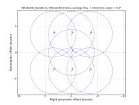
As it is shown in Figures 2 and 3 of IRAS16293Band9, these observations have a 7 pointing mosaic, which you can visualize with the next command (see also Figure 1).
# Make a plot of the mosaic pattern with field ids identified
aU.plotMosaic(vis='IRAS16293_Band9.ms',sourceid='0',
              doplot=True,figfile='mosaic_pattern.png')
You might wander what of these pointings or fields have stronger line emission. You can know this by running the next command. We set spw='1', and you can check all the plots for all the fields by just hitting the arrow for "next". Also see Figure 2 for an example of the output.
# See which mosaic fields have the brightest line emission
plotms(vis='IRAS16293_Band9.ms',
       field='',xaxis='uvdist', yaxis='amp',
       spw='1', avgchannel='3840',coloraxis='field',
       iteraxis='field')
Last checked on CASA Version 3.4.0.

