First Look at Line Imaging CASA 6.4
This guide is written for CASA 6.4.1.12 and uses Python 3.
This lesson steps you through imaging of spectral lines.
You should have downloaded the data package as part of the first imaging tutorial. If you haven't done that yet, check the First Look At Imaging CASA 6.4 Guide for instructions.
We start here with the self-calibrated data from the previous tutorial. We could just as easily begin with the non self-calibrated data, but we would not then benefit from the improvements that the self calibration provided.
Note that it often makes good sense to self-calibrate on the continuum source, even when the main science goal is to image spectral line emission. This is especially true when the continuum is bright and not overly complex. Sometimes, though, it can make better sense to self-calibrate on a spectral line, and apply those solutions to the entire data set. For now, we will apply the continuum self-cal solutions to our spectral line data to optimize our spectral line images.
First, copy the self-calibrated measurement set to the current directory. This measurement set contains both spectral line and continuum data for our science target. Note that if you would like to use your own self-calibrated measurement set from the previous tutorial here, you will need to change the filename from 'sis14_twhya_selfcal.ms' to your best result (i.e., 'sis14_twhya_selfcal_3.ms') throughout this tutorial.
# In CASA
os.system("rm -rf sis14_twhya_selfcal.ms")
os.system("tar -xvf ../working/sis14_twhya_selfcal.ms.tar")
The untarred measurement set will be automatically placed in your current directory, which can be verified with an "ls" command.
Continuum subtraction
Our first step is to remove the continuum emission from the UV data. Here, continuum emission means broadband emission that spans all spectral channels. The continuum may have some mild frequency dependence, and that's OK. The cleanest way to do the continuum subtraction is to operate on the UV data, fitting the amplitudes using only those spectral channels that are free from spectral line emission. We will do so using the CASA task uvcontsub.
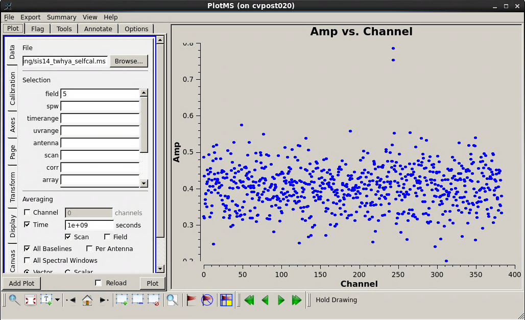
The main subtlety in the UV continuum subtraction is that we want to be sure to fit the continuum using only channels that contain mostly continuum (and not line) emission. To this end, the first thing that we will do is plot the integrated spectrum of the science target using the plotms task. We specify the science source (field 5) and plot the amplitude as a function of channel number, averaging the data over time. (The parameter avgscan=True tells CASA to allow time averaging across scans.)

# In CASA
plotms(vis='sis14_twhya_selfcal.ms',
       xaxis='channel',
       yaxis='amp',
       field='5',
       avgspw=False,
       avgtime='1e9',
       avgscan=True,
       avgbaseline=True,
       showgui = True)
Inside the plotms tabs, you can toggle the axis to frequency and then back to channel - the N2H+ line is at 372.67249 GHz and you can see that there are several high amplitudes around channel 250 representing a weak but still visible spectral line. The rest of the spectrum seems reasonably clear for measuring the continuum. To be sure that we exclude all spectral line emission, let's avoid channels 240-280 in our continuum fit.
In our call to uvcontsub, we specify the line-free regions by setting fitspw='0:0~239;281~383' and then set excludechans=False to tell CASA that these are the channels to fit. If you want to specify the region NOT to fit (where the line is), use excludechans=True. In this case we'll fit only a constant amplitude (flat) continuum by setting the fitorder to 0. We target only field '5', the science source. Note that we want to attempt this subtraction for every individual UV data point and so we request a solution interval equal to the integration time.
On a larger ALMA dataset, this step may take some time depending on your computing resources!
# In CASA
os.system('rm -rf sis14_twhya_selfcal.ms.contsub')
uvcontsub(vis = 'sis14_twhya_selfcal.ms',
          field = '5',
          fitspw = '0:0~239;281~383',
          excludechans = False,
          fitorder = 0,
          solint='int')
In CASA 6, you will see a warning that uvcontsub is using the original Visibility Iterator, which is the underlying iteration and retrieval mechanism used when processing visibility data. A new version of the Visibility Iterator has been developed and deployed in several other calibration tasks in CASA 5.0 and later (see CASA eNews for more information). We can ignore this warning.
WARN calibrater Forcing use of OLD VisibilityIterator.
The output is a continuum-subtracted UV data set that has the file extension ".contsub". We can now plot that using plotms, similar to what we did before, and look at the spectrum, which should now contain only the spectral line. Note that because we only ran uvcontsub on field '5' above, and created a new MS, the science data is now labeled as field '0' (the first and only field) in the new measurement set. (Run listobs on the continuum-subtracted data set to see how the field is now labeled, if you like.)

# In CASA
plotms(vis='sis14_twhya_selfcal.ms.contsub',
       xaxis='channel',
       yaxis='amp',
       field='0',
       avgspw=False,
       avgtime='1e9',
       avgscan=True,
       avgbaseline=True,
       showgui = True)
The continuum subtraction looks reasonably good. We'll see better when we image the cube.
Imaging the spectral line
Line imaging is like continuum imaging with (as you would expect) the additional dimension of spectral information. In the call to tclean, we now need to set specmode="cube". Further, we need to specify the third axis onto which the data will be gridded by setting appropriate values (and units) for the start, width, and nchan parameters. This third axis can be specified in units of channel, velocity, or frequency. Any of these choices would be valid for these data. Here, we image 15 channels in the output data cube, each 0.5 km/s in width, starting at 0 km/s in the LSRK reference frame by setting start="0.0km/s", nchan=15, and width="0.5km/s". The velocity is defined relative to the N2H+ rest frequency, which can be looked up in splatalogue.
Set the N2H+ rest frequency in a python variable as follows:
# In CASA
restfreq = '372.67249GHz'
Next we will use tclean to make the cube, targeting the continuum-subtracted data. Set field to '0' and spw to '0' (the only options in this data set), and use specmode="cube" with 15 channels of 0.5 km/s starting at 0.0 km/s defined in the LSRK frame (a common frame for Galactic and extragalactic work). We also set restoringbeam='common' to ensure a constant beam size for each plane in the cube. Weighting has been changed to 'briggsbwtaper'. This is a new weighting scheme available starting in CASA 6.2. See Imaging Algorithms for more information. In addition, the beam-fitting algorithm has been updated, starting in CASA 6.2. Otherwise, this tclean will resemble our previous calls when we imaged the continuum.

# In CASA
os.system('rm -rf twhya_n2hp.*')
tclean(vis = 'sis14_twhya_selfcal.ms.contsub',
       imagename = 'twhya_n2hp',
       field = '0',
       spw = '0',
       specmode = 'cube',
       perchanweightdensity=True,
       nchan = 15,
       start = '0.0km/s',
       width = '0.5km/s',
       outframe = 'LSRK',
       restfreq = restfreq,
       deconvolver= 'hogbom',
       gridder = 'standard',
       imsize = [250, 250],
       cell = '0.08arcsec',
       phasecenter = 0,
       weighting = 'briggsbwtaper',
       robust = 0.5,
       restoringbeam='common',
       interactive = True,
       niter=5000)
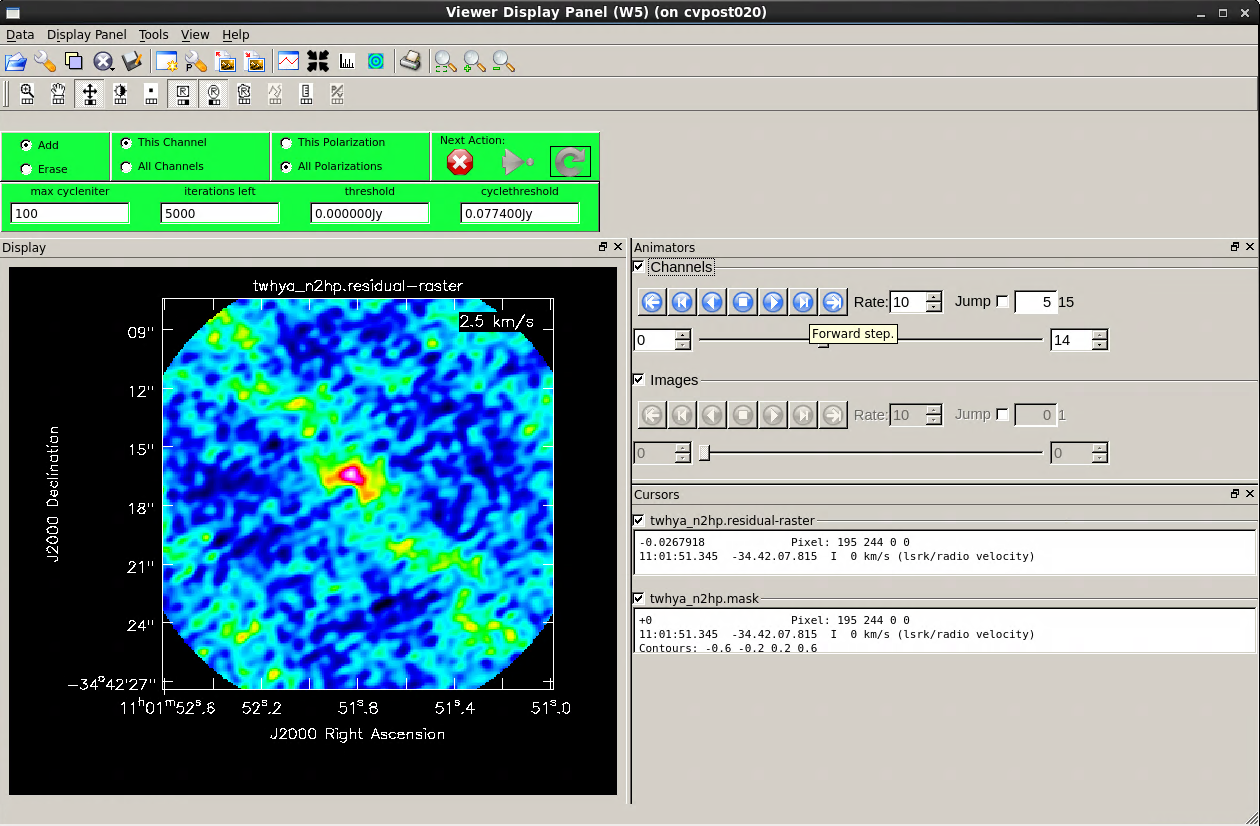
We specified interactive mode, so the clean GUI will come up. When it does, step through the channels in the cube using the tape deck controls. We see emission over a few channels near the center of the cube. Notice the location of the emission shifts from channel to channel -- Cool! This is showing velocity structure from the rotating disk!
Since the line emission has fairly low signal-to-noise, we don't expect cleaning to make a dramatic improvement here. But, let's give it a shot to try to improve the image. For spectral cubes, it's possible to specify a clean mask individually for each velocity channel, or you can specify a single mask that gets applied to all channels. There is a button at the top of the tclean GUI that toggles between these options. Both are viable approaches. For a high fidelity telescope like ALMA it's often (but not always) fine to use a single mask across all channels. Try interactively drawing a clean mask as you did previously in the CASA guide for continuum imaging. Select either the button to clean only "This channel" or apply the clean mask to all channels by selecting the "All channels" button below it. Then clean for 100 iterations or so until the maximum of the residuals inside the clean box is comparable to the surrounding noise. To finish, close the clean window by clicking the red "X."
The output of the tclean task is a data cube. You can use the viewer to inspect the cube, plot spectra, estimate the noise, and overlay this result with the earlier continuum image.

# In CASA
imview("twhya_n2hp.image")
At this point you should play with viewer. Change the velocity axis definitions, measure statistics from the image planes, and so on.
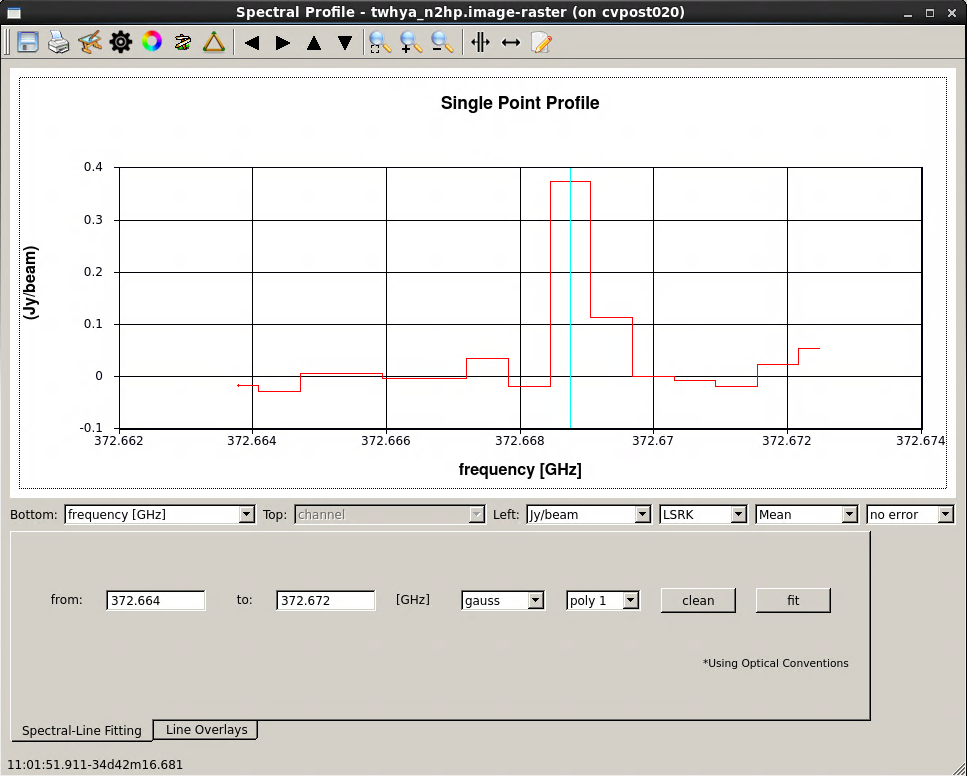
The viewer gives you the capability to make spectral profile plots. On the viewer GUI, select "Tools -> Spectral Profile ...". Then draw a box or ellipse around a region of interest, or set a single point using the "point marking" button to get a spectrum from a cut through a single pixel on the image. The figure here shows a spectrum from a single-pixel cut through the cube, with the pixel set on a lobe of bright spectral line emission.
Primary beam correction
As with continuum imaging, the line data cubes produced by CASA do not have the primary beam correction by default. Remember that to form an astronomically correct image of the sky, the output of tclean needs to be divided by this primary beam (or, in the case of mosaics, the combination of primary beam patterns used to make the mosaic). For final calculations you will therefore want to produce a primary beam-corrected version of your cube. You can create the primary beam-corrected cube in tclean by setting the parameter pbcor = True. This will produce an additional file with the extension .image.pbcor, which is the cleaned cube corrected for the primary beam.
If you've already cleaned your data and don't want to rerun tclean, CASA stores the primary beam information needed to make this correction in the file with the .pb extension. The CASA task impbcor can be used to combine the .pb image with the output image from tclean to produce a primary-beam corrected image. First remove the old primary beam corrected image if it exists:
# In CASA
os.system('rm -rf twhya_n2hp.pbcor.image')
Now correct the image:
# In CASA
impbcor(imagename='twhya_n2hp.image',
        pbimage='twhya_n2hp.pb',
        outfile='twhya_n2hp.pbcor.image')