EVLA high frequency spectral line tutorial - IRC+10216 - calibration
This page is under development
This CASA Guide provides a simplified approach to the editing, calibration, and imaging of a galactic EVLA observation for use in NRAO Community Day Events. For a complete description of the data reduction process see EVLA high frequency Spectral Line tutorial - IRC+10216 part1 and EVLA high frequency Spectral Line tutorial - IRC+10216 part2.
Overview
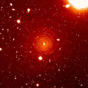
This tutorial describes the data reduction for two spectral lines, HC3N and SiS, observed toward the AGB star IRC+10216 by the EVLA in D-configuration.
Getting the data
The data for this tutorial can be obtained by anonymous FTP from ftp://ftp.aoc.nrao.edu/staff/gvanmoor/community_day/. Download all 4 TAR files.
For example,
# In UNIX
wget 'ftp://ftp.aoc.nrao.edu/staff/gvanmoor/community_day/*'
Initial Inspection and Flagging
GEt a summary listing of the data set using listobs.
# In CASA
vis = 'day2_TDEM0003_20s_full'
listobs(vis=vis, verbose=True)
Below we have cut and pasted the most relevant output from the logger.
Fields: 4
  ID   Code Name                RA              Decl          Epoch   SrcId nVis
  2    D    J0954+1743          09:54:56.82363 +17.43.31.2224 J2000   2     32726
  3    NONE IRC+10216           09:47:57.38200 +13.16.40.6600 J2000   3     99540
  5    F    J1229+0203          12:29:06.69973 +02.03.08.5982 J2000   5     5436
  7    E    J1331+3030          13:31:08.28798 +30.30.32.9589 J2000   7     2736
   (nVis = Total number of time/baseline visibilities per field)
Spectral Windows:  (2 unique spectral windows and 1 unique polarization setups)
  SpwID  #Chans Frame Ch1(MHz)    ChanWid(kHz)  TotBW(kHz)  Corrs
  0          64 TOPO  36387.2295  125           8000        RR  RL  LR  LL
  1          64 TOPO  36304.542   125           8000        RR  RL  LR  LL
Sources: 10
  ID   Name                SpwId RestFreq(MHz)  SysVel(km/s)
  0    J1008+0730          0     0.03639232     -0.026
  0    J1008+0730          1     0.03639232     -0.026
  2    J0954+1743          0     0.03639232     -0.026
  2    J0954+1743          1     0.03639232     -0.026
  3    IRC+10216           0     0.03639232     -0.026
  3    IRC+10216           1     0.03639232     -0.026
  5    J1229+0203          0     0.03639232     -0.026
  5    J1229+0203          1     0.03639232     -0.026
  7    J1331+3030          0     0.03639232     -0.026
  7    J1331+3030          1     0.03639232     -0.026
Antennas: 19:
  ID   Name  Station   Diam.    Long.         Lat.
  0    ea01  W09       25.0 m   -107.37.25.2  +33.53.51.0
  1    ea02  E02       25.0 m   -107.37.04.4  +33.54.01.1
  2    ea03  E09       25.0 m   -107.36.45.1  +33.53.53.6
  3    ea04  W01       25.0 m   -107.37.05.9  +33.54.00.5
  4    ea05  W08       25.0 m   -107.37.21.6  +33.53.53.0
  5    ea07  N06       25.0 m   -107.37.06.9  +33.54.10.3
  6    ea08  N01       25.0 m   -107.37.06.0  +33.54.01.8
  7    ea09  E06       25.0 m   -107.36.55.6  +33.53.57.7
  8    ea12  E08       25.0 m   -107.36.48.9  +33.53.55.1
  9    ea15  W06       25.0 m   -107.37.15.6  +33.53.56.4
  10   ea19  W04       25.0 m   -107.37.10.8  +33.53.59.1
  11   ea20  N05       25.0 m   -107.37.06.7  +33.54.08.0
  12   ea21  E01       25.0 m   -107.37.05.7  +33.53.59.2
  13   ea22  N04       25.0 m   -107.37.06.5  +33.54.06.1
  14   ea23  E07       25.0 m   -107.36.52.4  +33.53.56.5
  15   ea24  W05       25.0 m   -107.37.13.0  +33.53.57.8
  16   ea25  N02       25.0 m   -107.37.06.2  +33.54.03.5
  17   ea27  E03       25.0 m   -107.37.02.8  +33.54.00.5
  18   ea28  N08       25.0 m   -107.37.07.5  +33.54.15.8
We summarize the observing strategy in this table.
| Gain calibrator | J0954+1743 | field id = 2 |
|---|---|---|
| Bandpass calibrator | J1229+0203 | field id = 5 |
| Flux calibrator | J1331+3030 (3C286) | field id = 7 |
| Science target | IRC+10216 | field id = 3 |
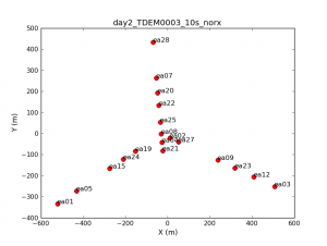
Create a plot of antenna positions using plotants.
# In CASA
plotants(vis=vis)
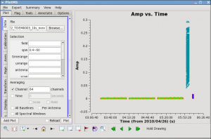
Next, let's look at all the source amplitudes as a function of time using plotms.
# In CASA
plotms(vis=vis, xaxis='time', yaxis='amp', correlation='RR,LL',
       avgchannel='64', spw='0:4~60', coloraxis='field')
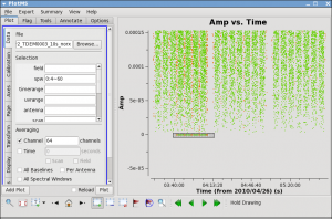
Now zoom in on the region very near zero amplitude for sources J0954+1743 and IRC+10216. To zoom, select the Zoom tool in lower left corner of the plotms GUI, then you can left click to draw a box. Look for the low values (you may want to zoom a few times to really see the suspect points clearly). Now use the Mark Region and Locate buttons (located along the bottom of the GUI) to see which antenna is causing problems. The output will be shown in the logger. Since all the "located" baselines include ea12, this is the responsible antenna.
Now click the clear region button, and then go back to the zoom button to zoom in further to note exactly what the time range is: 03:41:00~04:10:00.
Check the other sideband by changing spw to 1:4~60. You will have to rezoom. If you have trouble, click on the Mark icon and then back to zoom. In spw=1, ea07 is bad from the beginning until after next pointing run: 03:21:40~04:10:00. To see this, compare the amplitudes when antenna is set to 'ea07' and when it is set to one of the other antennas, such as 'ea08'.
If you set antenna to 'ea12' and zoom in on this intial timerange, you can also see that ea12 is bad during the same time range as for spw 0. You can also see this by entering '!ea07' for antenna, which removes ea07 from the plot (in CASA selection, ! deselects).
We can flag the bad data using flagdata.
# In CASA
flagdata(vis=vis,
         field=['2,3','2,3'],
         spw=['','1'],
         antenna=['ea12','ea07'],
         timerange=['03:41:00~04:10:00','03:21:40~04:10:00'])
flagdata works by spanning up a matrix. The first entries in each list must be taken as one flagging command, as well as the second entries etc. Lists within lists are fine. In the above example, the first flagging command is issued for fields 2 and 3 for all spws and within the 03:41:00~04:10:00 timerange. A second command is again for the fields 2 and 3 but for spw 1 only and for the second timerange in the list '03:21:40~04:10:00'.
Note that because the chosen timerange is limited to fields 2 and 3, the field parameter is not really needed; however, flagdata will run fastest if you put as many constraints as possible.
Set Up the Model for the Flux Calibrator
We set the model for the flux calibrator using setjy. First, check the availability of calibration models.
# In CASA
setjy(vis=vis,listmodimages=T)
There is no Ka-band model of 3C286. We will use the K-band model instead.
# In CASA
setjy(vis=vis,field='7',spw='0~1',
      modimage='3C286_K.im')
setjy scales the total flux in the model image to that appropriate for your individual spectral window frequencies according to the calibrator's flux and reports this number to the logger.
The logger output for each spw is:
J1331+3030 (fld ind 7) spw 0  [I=1.7762, Q=0, U=0, V=0] Jy, (Perley-Butler 2010)
J1331+3030 (fld ind 7) spw 1  [I=1.7794, Q=0, U=0, V=0] Jy, (Perley-Butler 2010)
The absolute fluxes for the frequencies have now been determined and one can proceed to the bandpass and complex gain calibrations.
Bandpass Calibration
Correct the phase variations with time before solving for the bandpass to prevent decorrelation of the vector averaged bandpass solution.
# In CASA
gaincal(vis=vis, caltable='bpphase.gcal', field='5', spw='0~1:20~40',
        refant='ea02', gaintype='G', calmode='p',solint='int',
        gaincurve=T)
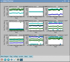
Plot the solutions using plotcal.
# In CASA
plotcal(caltable='bpphase.gcal',xaxis='time',yaxis='phase',
        iteration='antenna',subplot=331,plotrange=[0,0,-180,180])
Next we can apply this phase solution on the fly while determining the bandpass solutions on the timescale of the bandpass calibrator scan (solint='inf').
# In CASA
bandpass(vis=vis, caltable='bandpass.bcal', field='5', refant='ea02',
         solint='inf', solnorm=T, gaintable='bpphase.gcal',
         gaincurve=T)
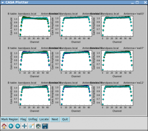
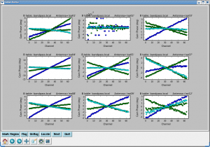
Plot the solutions, amplitude and phase:
# In CASA
plotcal(caltable='bandpass.bcal',xaxis='chan',yaxis='amp',
        iteration='antenna',subplot=331)
# In CASA
plotcal(caltable='bandpass.bcal',xaxis='chan',yaxis='phase',
        iteration='antenna',subplot=331)
Remaining Calibration
In this Community Day Event guide, we will skip over the remaining calibration steps. However, you can refer to EVLA high frequency Spectral Line tutorial - IRC+10216 part1 for full details. To summarize the missing steps, you bootstrap the flux densities of the secondary calibrators by
- doing a phase only calibration on all calibrators using gaincal,
- doing amplitude only calibration on all calibrators while applying the phase-only solutions, and
- deriving the flux density of the secondary calibrators while applying the previously obtained solutions.
Then, you can calibrate the target source using the phase and amplitude solutions you have obtained. Apply the target source calibration solutions using applycal. Use plotms to examine the calibrated data. If more flagging is required, redo all calibration steps. When the data look good, split the target source into a separate measurement set. Subtract the continuum flux using uvcontsub. Make Doppler corrections using cvel, or let clean do the Doppler corrections on the fly.
This tutorial picks up where EVLA high frequency spectral line tutorial - IRC+10216 - calibration leaves off.
Imaging
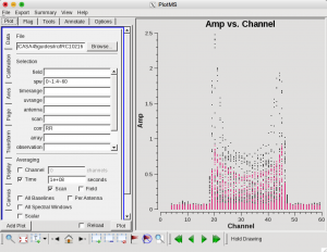
The continuum-subtracted spectral line data is contained in IRC10216_spls.ms. Use plotms to plot the lines.
plotms(vis='IRC10216_spls.ms', xaxis='channel', yaxis='amp',
       avgtime='1e8', avgscan=T, coloraxis='spw')
Now it is time to image the visibility data using clean. For illustration, we will clean channel 22 of the SiS line.
# In CASA
clean(vis='IRC10216_spls.ms', imagename='ch22', spw='1:22~22',
      mode='channel', nchan=1, start='', width=1, niter=100000,
      gain=0.1, threshold='3.0mJy', psfmode='clark', imagermode='csclean',
      interactive=T, npercycle=100, imsize=300, cell=['0.4arcsec', '0.4arcsec'],
      stokes='I', weighting='briggs', robust=0.5)
After running the above command, make a region in the CASA viewer. Double-click inside the region and clean by clicking the green circular arrow. After each cycle, click the green circular arrow again if the flux inside the region is brighter than the flux peaks outside the region. When you are finished cleaning, click the red 'STOP' button.
Open the resulting image using the viewer.
# In CASA
viewer("ch22.image")
In the viewer, make a region and click inside it to get statistics about the portion of the image in the region.
Analyze the Image Cubes
Open the HC3N image cube in the viewer.
# In CASA
viewer("IRC10216_HC3N.image")
Click the 'Play' button to view all channels in the cube. Select Tool --> Spectral profile... from the pull down menu. Create a region on the image to view the spectrum within the region.
Open the SiS image cube in the viewer.
# In CASA
viewer("IRC10216_SiS.image")
Determine what channels in the cube have emission. Then make moment maps using immoments.
# In CASA
immoments(imagename="IRC10216_SiS.image", moments=[0], axis="spectral",
          chans="12~40", outfile="IRC10216_Sis.mom0")
Open the moment map in the viewer.
# In CASA
viewer("IRC10216_Sis.mom0")
Overlay contours by selecting Data --> Open from the pull down menu, selecting the moment-0 map, and clicking 'contour map'.
Last checked on CASA Version 3.3.0.
