Averaging data in plotms: Difference between revisions
No edit summary |
No edit summary |
||
| (19 intermediate revisions by 2 users not shown) | |||
| Line 1: | Line 1: | ||
You can average your measurement set on the fly with | [[Category: CASA Basics]][[Category: Interactive Tools]] | ||
{{Interactive Tools Intro}} | |||
__FORCETOC__ | |||
You can average your measurement set on the fly with {{plotms}}. The '''averaging''' options can be found under the Data tab. | |||
{|vspace="100" | {|vspace="100" | ||
| Line 5: | Line 10: | ||
|- | |- | ||
| | | | ||
== Time Averaging == | |||
<div style="float: left; width: 50%; align: left;"> | <div style="float: left; width: 50%; align: left;"> | ||
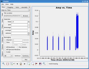
Time averaging can be a little tricky, as it is controlled by three fields. If you click the checkbox next to '''Time''' under '''Averaging''', a blank box with units of 'seconds' should become active, along with two checkboxes: '''Scan''' and '''Field'''. To the right, we've plotted two calibrator sources from a multi-source measurement set. There has been no averaging. One is a phase calibrator observed in six scans, while the other is a brighter flux calibrator observed in one scan at the end of the observations. | |||
</div> | |||
<div style="float: right; width: 50%; text-align: center;"> | |||
[[File:plotms_timeave0.jpg | 300px]] | |||
''Click to enlarge'' | |||
</div> | |||
|- style="background-color:#eeeeee;" | |||
| | |||
<div style="float: left; width: 50%; align: left;"> | |||
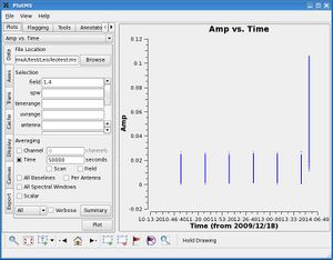
Try setting the blank box to a very long time---let's say 50000 seconds---much longer than your total time observing. If we plot amplitude vs. time, you'll notice that not all of the data has been averaged together in time; in fact, only data within individual scans has been averaged together. | |||
</div> | </div> | ||
<div style="float: right; width: 50%; text-align: center;"> | <div style="float: right; width: 50%; text-align: center;"> | ||
[[File: | [[File:plotms_timeave1.jpg | 300px]] | ||
''Click to enlarge'' | |||
</div> | |||
|- | |||
| | |||
<div style="float: left; width: 50%; align: left;"> | |||
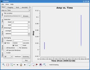
If we click on the '''Scan''' checkbox and replot the data, we now see that the scans for the individual calibrators have been averaged together. | |||
</div> | |||
<div style="float: right; width: 50%; text-align: center;"> | |||
[[File:plotms_timeave2.jpg | 300px]] | |||
''Click to enlarge'' | ''Click to enlarge'' | ||
| Line 21: | Line 52: | ||
| | | | ||
<div style="float: left; width: 50%; align: left;"> | |||
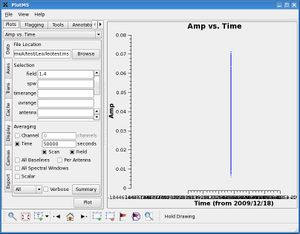
Finally, if for some reason, we'd like to average the two sources together in time, we click to make a checkmark in the '''Fields''' box. Now we get a plot like the one to the right; all data from both calibrators has been averaged to a single point in time. | |||
Note that if we had inputted a relatively short time into the '''Time''' blank box---say, 60 seconds---clicking the '''Scan''' or '''Field''' box would have no impact. This is because this time is shorter than individual scans and is shorter than the time between visits to different fields. | |||
</div> | |||
<div style="float: right; width: 50%; text-align: center;"> | |||
[[File:plotms_timeave3.jpg | 300px]] | |||
''Click to enlarge'' | |||
</div> | |||
|- | |||
| | |||
== Other Averaging == | |||
Once you understand time averaging, the other '''Averaging''' options are quite intuitive. You can average channels together if you click the box next to '''Channel''' and fill in the blank box with a number greater than 1. You can also average across spectral windows by checking the box next to '''All Spectral Windows''' (This will average together all channel 1s from all windows to make an averaged channel 1, etc; IS THIS TRUE?). | |||
You can average all baselines in the dataset together by clicking '''All Baselines''' (in which case, if you plotted amplitude vs. baseline, there would only be one data point along the x axis), or you can average '''Per Antenna''' (and then, if you plotted amplitude vs. baseline, there should be as many data points along the x axis as there are antennae). | |||
Finally, note that all of this is, by default, vector averaging. If you would prefer scalar averaging, check the box next to '''Scalar'''. | |||
Last checked on CASA Version 3.0.1 (r10380). | |||
--[[User:Lchomiuk|Laura Chomiuk]] 01:25, 19 February 2010 (UTC) | |||
Latest revision as of 17:58, 7 June 2010
You can average your measurement set on the fly with plotms. The averaging options can be found under the Data tab.
Time AveragingTime averaging can be a little tricky, as it is controlled by three fields. If you click the checkbox next to Time under Averaging, a blank box with units of 'seconds' should become active, along with two checkboxes: Scan and Field. To the right, we've plotted two calibrator sources from a multi-source measurement set. There has been no averaging. One is a phase calibrator observed in six scans, while the other is a brighter flux calibrator observed in one scan at the end of the observations. |
|
Try setting the blank box to a very long time---let's say 50000 seconds---much longer than your total time observing. If we plot amplitude vs. time, you'll notice that not all of the data has been averaged together in time; in fact, only data within individual scans has been averaged together. |
|
If we click on the Scan checkbox and replot the data, we now see that the scans for the individual calibrators have been averaged together. |
|
Finally, if for some reason, we'd like to average the two sources together in time, we click to make a checkmark in the Fields box. Now we get a plot like the one to the right; all data from both calibrators has been averaged to a single point in time. Note that if we had inputted a relatively short time into the Time blank box---say, 60 seconds---clicking the Scan or Field box would have no impact. This is because this time is shorter than individual scans and is shorter than the time between visits to different fields. |
Other AveragingOnce you understand time averaging, the other Averaging options are quite intuitive. You can average channels together if you click the box next to Channel and fill in the blank box with a number greater than 1. You can also average across spectral windows by checking the box next to All Spectral Windows (This will average together all channel 1s from all windows to make an averaged channel 1, etc; IS THIS TRUE?). You can average all baselines in the dataset together by clicking All Baselines (in which case, if you plotted amplitude vs. baseline, there would only be one data point along the x axis), or you can average Per Antenna (and then, if you plotted amplitude vs. baseline, there should be as many data points along the x axis as there are antennae). Finally, note that all of this is, by default, vector averaging. If you would prefer scalar averaging, check the box next to Scalar.
--Laura Chomiuk 01:25, 19 February 2010 (UTC) |


