Antennae Band7 - Calibration for CASA 3.3
- This script assumes that you have downloaded Antennae_Band7_UnCalibratedMSAndTablesForReduction.tgz from AntennaeBand7#Obtaining_the_Data
- Details of the ALMA observations are provided at AntennaeBand7
- This portion of the guide covers calibration of the raw visibility data. To skip to the imaging portion of the guide, see: Antennae Band7 - Imaging.
Unpack the Data
Once you have downloaded the Antennae_Band7_UnCalibratedMSandTablesForReduction.tgz, unpack the file in a terminal outside CASA using
>tar -xvzf Antennae_Band7_UnCalibratedMSandTablesForReduction.tgz
then change directory (cd) to the directory Antennae_Band7_UnCalibratedMSandTablesForReduction.
You may wish to type
>ls
to look at the files present. You should see a bunch of files with extension ".ms" indicating that these are CASA measurement set (MS) files. The data have already been converted to MS format using the CASA task importasdm. Accompanying the data are some basic calibration tables holding system temperature (Tsys) and water vapor radiometer (WVR) information that we have generated outside of CASA (for Early Science, CASA will be able to generate these tables).
To begin, start CASA by typing
>casapy
Initial Inspection
First we will take stock of what we have. If you have not already done so, begin by reviewing the description of the observations here: AntennaeBand7. The 10 data sets each target either the northern or the southern mosaic, as follows:
Northern Mosaic:
- uid___A002_X1ff7b0_Xb.ms
- uid___A002_X207fe4_X3a.ms
- uid___A002_X207fe4_X3b9.ms
- uid___A002_X2181fb_X49.ms
Southern Mosaic:
- uid___A002_X1ff7b0_X1c8.ms
- uid___A002_X207fe4_X1f7.ms
- uid___A002_X207fe4_X4d7.ms
- uid___A002_X215db8_X18.ms
- uid___A002_X215db8_X1d5.ms
- uid___A002_X215db8_X392.ms
The first step is to get basic information about the data: targets observed, time range, spectral setup, and so on. We do this using the task listobs, which will output a detailed summary of each dataset. Enter the following commands into CASA:
# In CASA

# Define a python list holding the names of all of our data sets
basename_all=["uid___A002_X1ff7b0_Xb","uid___A002_X207fe4_X3a","uid___A002_X207fe4_X3b9",
     "uid___A002_X2181fb_X49","uid___A002_X1ff7b0_X1c8","uid___A002_X207fe4_X1f7",
     "uid___A002_X207fe4_X4d7","uid___A002_X215db8_X18","uid___A002_X215db8_X1d5",
     "uid___A002_X215db8_X392"]

# Loop over each element in the list and create summary file using listobs
for asdm in basename_all:
        listobs(vis=asdm+'.ms', listfile=asdm+'.listobs.txt', verbose=True)
Note that after cutting and pasting a 'for' loop like this you often have to press return twice to execute. You may also want to take care to paste a line at a time if you are having trouble copy and pasting. Alternatively, you can try "cpaste" to paste blocks of code. To do so type "cpaste" at the CASA prompt, paste your commands, and then type "--" and hit return on the final (otherwise empty) line. This should look something like this:
CASA <8>: cpaste
Pasting code; enter '--' alone on the line to stop.
:basename_all=["uid___A002_X1ff7b0_Xb","uid___A002_X207fe4_X3a","uid___A002_X207fe4_X3b9",
:     "uid___A002_X2181fb_X49","uid___A002_X1ff7b0_X1c8","uid___A002_X207fe4_X1f7",
:     "uid___A002_X207fe4_X4d7","uid___A002_X215db8_X18","uid___A002_X215db8_X1d5",
:     "uid___A002_X215db8_X392"]
:
:for asdm in basename_all:
:    print asdm
:--
uid___A002_X1ff7b0_Xb
uid___A002_X207fe4_X3a
uid___A002_X207fe4_X3b9
uid___A002_X2181fb_X49
uid___A002_X1ff7b0_X1c8
uid___A002_X207fe4_X1f7
uid___A002_X207fe4_X4d7
uid___A002_X215db8_X18
uid___A002_X215db8_X1d5
uid___A002_X215db8_X392

CASA <9>:
If you have trouble, just carefully paste one line at a time directly into CASA and hit return until the desired command executes.
These commands define a python list called "basename_all", which contains the name of all 10 MS files. The "for" loop executes for each element in basename_all, calling listobs and directing the output to a file called, e.g., "uid___A002_X1ff7b0_Xb.listobs.txt" for the first measurement set.
You can browse through the listobs output as you would normally look at a text file (use emacs, vi, or another editor). You can also send the output to the terminal from inside of CASA. To do so type:
# In CASA
cat uid___A002_X1ff7b0_Xb.listobs.txt
or
# In CASA
os.system('more uid___A002_X1ff7b0_Xb.listobs.txt')
CASA knows a few basic shell commands like 'cat', 'ls', and 'rm' but for more complex commands you will need to run them inside 'os.system("command")'. For more information see http://casa.nrao.edu/ .
Here is an example of the (abridged) output from listobs for the first dataset in the list, uid___A002_X1ff7b0_Xb.ms, which targets the Northern Mosaic:
=============================================================================
 MeasurementSet Name:/Users/despada/Desktop/Imaging/Antennae/Datasets/band7/uid___A002_X1ff7b0_Xb.ms
=============================================================================
   Observer: Unknown     Project: T.B.D.
Observation: ALMA(11 antennas)
Data records: 181357       Total integration time = 4931.71 seconds
   Observed from   28-May-2011/01:25:27.6   to   28-May-2011/02:47:39.3 (UTC)
Fields: 26
  ID   Code Name         RA            Decl           Epoch   SrcId
  0    none 3c279        12:56:11.1666 -05.47.21.5247 J2000   0
  1    none Titan        12:42:43.9481 -01.43.38.3190 J2000   1
  2    none NGC4038 - A* 12:01:53.1701 -18.52.37.9200 J2000   2
  3    none NGC4038 - A* 12:01:51.9030 -18.51.49.9437 J2000   2
  4    none NGC4038 - A* 12:01:52.4309 -18.51.49.9437 J2000   2
  5    none NGC4038 - A* 12:01:52.9587 -18.51.49.9437 J2000   2
  6    none NGC4038 - A* 12:01:53.4866 -18.51.49.9436 J2000   2
  7    none NGC4038 - A* 12:01:54.0144 -18.51.49.9436 J2000   2
  8    none NGC4038 - A* 12:01:52.1669 -18.51.56.4319 J2000   2
  9    none NGC4038 - A* 12:01:52.6948 -18.51.56.4318 J2000   2
  10   none NGC4038 - A* 12:01:53.2226 -18.51.56.4318 J2000   2
  11   none NGC4038 - A* 12:01:53.7505 -18.51.56.4318 J2000   2
  12   none NGC4038 - A* 12:01:51.9030 -18.52.02.9201 J2000   2
  13   none NGC4038 - A* 12:01:52.4309 -18.52.02.9200 J2000   2
  14   none NGC4038 - A* 12:01:52.9587 -18.52.02.9200 J2000   2
  15   none NGC4038 - A* 12:01:53.4866 -18.52.02.9200 J2000   2
  16   none NGC4038 - A* 12:01:54.0144 -18.52.02.9199 J2000   2
  17   none NGC4038 - A* 12:01:52.1669 -18.52.09.4082 J2000   2
  18   none NGC4038 - A* 12:01:52.6948 -18.52.09.4082 J2000   2
  19   none NGC4038 - A* 12:01:53.2226 -18.52.09.4082 J2000   2
  20   none NGC4038 - A* 12:01:53.7505 -18.52.09.4081 J2000   2
  21   none NGC4038 - A* 12:01:51.9030 -18.52.15.8964 J2000   2
  22   none NGC4038 - A* 12:01:52.4309 -18.52.15.8964 J2000   2
  23   none NGC4038 - A* 12:01:52.9587 -18.52.15.8963 J2000   2
  24   none NGC4038 - A* 12:01:53.4866 -18.52.15.8963 J2000   2
  25   none NGC4038 - A* 12:01:54.0144 -18.52.15.8963 J2000   2
   (nVis = Total number of time/baseline visibilities per field)
Spectral Windows:  (9 unique spectral windows and 2 unique polarization setups)
  SpwID  #Chans Frame Ch1(MHz)    ChanWid(kHz)TotBW(kHz)  Ref(MHz)    Corrs
  0           4 TOPO  184550      1500000     7500000     183300      I
  1        3840 TOPO  344845.586  488.28125   1875000     344908.33   XX  YY
  2           1 TOPO  343908.086  1875000     1875000     344908.33   XX  YY
  3        3840 TOPO  356845.586  488.28125   1875000     344908.33   XX  YY
  4           1 TOPO  343908.086  1875000     1875000     344908.33   XX  YY
  5         128 TOPO  344900.518  15625       2000000     344908.33   XX  YY
  6           1 TOPO  343892.705  1796875     1796875     344908.33   XX  YY
  7         128 TOPO  356900.518  15625       2000000     344908.33   XX  YY
  8           1 TOPO  343892.705  1796875     1796875     344908.33   XX  YY

Antennas: 11 'name'='station'
   ID=   0-3: 'DV02'='A015', 'DV04'='J505', 'DV06'='T704', 'DV07'='A004',
   ID=   4-7: 'DV08'='A072', 'DV09'='A008', 'DV10'='A009', 'DV11'='A016',
   ID=  8-10: 'PM01'='T702', 'PM02'='A017', 'PM03'='J504'
================================================================================
And here is an example of the listobs for uid___A002_X1ff7b0_X1c8.ms, which targets the Southern Mosaic:
================================================================================
           MeasurementSet Name:  /export/lustre/aleroy/Antennae_Band7_UnCalibratedMSandTablesForReduction/uid___A002_X1ff7b0_X1c8.ms      MS Version 2
================================================================================
   Observer: Unknown     Project: T.B.D.
Observation: ALMA
Data records: 175615       Total integration time = 4927.1 seconds
   Observed from   28-May-2011/02:50:18.2   to   28-May-2011/04:12:25.3 (UTC)

Fields: 33
  ID   Code Name                RA              Decl          Epoch   SrcId nVis
  0    none 3c279               12:56:11.16657 -05.47.21.5247 J2000   0     12232
  1    none Titan               12:42:44.82765 -01.43.41.4224 J2000   1     10615
  2    none 3c279               12:56:11.16600 -05.47.21.5250 J2000   2     27764
  3    none Antennae            12:01:53.17008 -18.52.37.9200 J2000   3     4829
  4    none Antennae            12:01:52.18699 -18.53.30.3952 J2000   3     3883
  5    none Antennae            12:01:52.64413 -18.53.26.6494 J2000   3     3883
  6    none Antennae            12:01:53.10127 -18.53.22.9035 J2000   3     3872
  7    none Antennae            12:01:53.55841 -18.53.19.1577 J2000   3     4818
  8    none Antennae            12:01:54.01554 -18.53.15.4119 J2000   3     4829
  9    none Antennae            12:01:54.47268 -18.53.11.6661 J2000   3     4829
  10   none Antennae            12:01:54.92982 -18.53.07.9203 J2000   3     3872
  11   none Antennae            12:01:55.38696 -18.53.04.1744 J2000   3     3883
  12   none Antennae            12:01:55.84409 -18.53.00.4286 J2000   3     4840
  13   none Antennae            12:01:56.30123 -18.52.56.6828 J2000   3     4818
  14   none Antennae            12:01:52.18700 -18.53.22.9033 J2000   3     4829
  15   none Antennae            12:01:52.64414 -18.53.19.1575 J2000   3     4818
  16   none Antennae            12:01:53.10128 -18.53.15.4116 J2000   3     4818
  17   none Antennae            12:01:53.55842 -18.53.11.6658 J2000   3     4840
  18   none Antennae            12:01:54.01555 -18.53.07.9200 J2000   3     3872
  19   none Antennae            12:01:54.47269 -18.53.04.1742 J2000   3     4829
  20   none Antennae            12:01:54.92983 -18.53.00.4284 J2000   3     4829
  21   none Antennae            12:01:55.38697 -18.52.56.6825 J2000   3     4829
  22   none Antennae            12:01:55.84410 -18.52.52.9367 J2000   3     4829
  23   none Antennae            12:01:51.72988 -18.53.19.1572 J2000   3     4818
  24   none Antennae            12:01:52.18702 -18.53.15.4114 J2000   3     4829
  25   none Antennae            12:01:52.64415 -18.53.11.6656 J2000   3     4829
  26   none Antennae            12:01:53.10129 -18.53.07.9197 J2000   3     2266
  27   none Antennae            12:01:53.55843 -18.53.04.1739 J2000   3     2266
  28   none Antennae            12:01:54.01557 -18.53.00.4281 J2000   3     3212
  29   none Antennae            12:01:54.47270 -18.52.56.6823 J2000   3     3234
  30   none Antennae            12:01:54.92984 -18.52.52.9365 J2000   3     3212
  31   none Antennae            12:01:55.38698 -18.52.49.1906 J2000   3     2266
  32   none Antennae            12:01:55.84411 -18.52.45.4448 J2000   3     3223
   (nVis = Total number of time/baseline visibilities per field)
Spectral Windows:  (9 unique spectral windows and 2 unique polarization setups)
  SpwID  #Chans Frame Ch1(MHz)    ChanWid(kHz)  TotBW(kHz)  Corrs
  0           4 TOPO  184550      1500000       7500000     I
  1        3840 TOPO  344845.586  488.28125     1875000     XX  YY
  2           1 TOPO  343908.086  1875000       1875000     XX  YY
  3        3840 TOPO  356845.586  488.28125     1875000     XX  YY
  4           1 TOPO  343908.086  1875000       1875000     XX  YY
  5         128 TOPO  344900.518  15625         2000000     XX  YY
  6           1 TOPO  343892.705  1796875       1796875     XX  YY
  7         128 TOPO  356900.518  15625         2000000     XX  YY
  8           1 TOPO  343892.705  1796875       1796875     XX  YY
Antennas: 11:
  ID   Name  Station   Diam.    Long.         Lat.
  0    DV02  A015      12.0 m   -067.45.15.3  -22.53.26.0
  1    DV04  J505      12.0 m   -067.45.18.0  -22.53.22.8
  2    DV06  T704      12.0 m   -067.45.16.2  -22.53.22.1
  3    DV07  A004      12.0 m   -067.45.15.9  -22.53.28.0
  4    DV08  A072      12.0 m   -067.45.12.6  -22.53.24.0
  5    DV09  A008      12.0 m   -067.45.15.4  -22.53.26.8
  6    DV10  A009      12.0 m   -067.45.16.1  -22.53.26.1
  7    DV11  A016      12.0 m   -067.45.16.4  -22.53.25.1
  8    PM01  T702      12.0 m   -067.45.18.6  -22.53.24.1
  9    PM02  A017      12.0 m   -067.45.15.9  -22.53.26.8
  10   PM03  J504      12.0 m   -067.45.17.0  -22.53.23.0
This output shows that three sources were observed in each data set: 3c279, Titan, and the Antennae.
- The Antennae are our science target. Note that the source name changes between the Northern Mosaic (where it is "NGC4038 - Antennae") and the Southern Mosaic (where it is just "Antennae") and that the source corresponds to a number of individual fields (the field id column). These are the individual mosaic pointings. There are 23 for the Northern Mosaic and 29 for the Southern Mosaic.
- Titan will be used to set the absolute flux scale of the data.
- 3c279 plays two roles: it will serve as our bandpass calibrator, to characterize the frequency response of the telescopes, and as our phase calibrator, to track changes in the phase and amplitude response of the telescopes over time. Observations of 3c279 are interleaved with observations of the Antennae.
The output also shows that the data contain many spectral windows, using the labeling scheme in the listobs above. These are:
- spw 0 targets ~185 GHz and holds water vapor radiometer data
- spw 1 and spw 3 hold our science data. These are "Frequency Domain Mode" (FDM) data with small (0.49 MHz) channel width and wide (1.875 GHz) total bandwidth. As a result these have a lot of channels (3840). spw 1 holds the lower sideband (LSB) data and includes the CO(3-2) line. We will focus on these data. For the CO(3-2) line the channel width corresponds to 0.426 km/s and the bandwidth of spw 1 to 1634 km/s.
- spw 2 and spw 4 hold frequency-averaged versions of spw 1 and 3 ("Channel 0" for those familiar with AIPS). These are used for quick inspection. We will not use them here.
- spw 5 and spw 7 hold lower resolution processing ("Time Domain Mode", TDM) data for the same part of the spectrum (baseband) as spws 1 and 3. These data have only 128 channels across 2 GHz bandwidth and so have a much coarser channel spacing than the FDM data. These were used to generate the calibration tables that we include in the tarball but will not otherwise appear in this guide.
The final column of the listobs output in the logger (not shown above) gives the scan intent. Later we will use this information to flag the pointing scans and the hot and ambient load calibration scans.
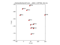
We'll now have a look at the configuration of the antennas used to take the data using the task plotants (Figure 1).
# In CASA
basename_all=["uid___A002_X1ff7b0_Xb","uid___A002_X207fe4_X3a","uid___A002_X207fe4_X3b9",
     "uid___A002_X2181fb_X49","uid___A002_X1ff7b0_X1c8","uid___A002_X207fe4_X1f7",
     "uid___A002_X207fe4_X4d7","uid___A002_X215db8_X18","uid___A002_X215db8_X1d5",
     "uid___A002_X215db8_X392"]

for asdm in basename_all:
    print "Antenna configuration for : "+asdm
    plotants(vis=asdm+'.ms', figfile=asdm+'.plotants.png')
    dummy_string = raw_input("Hit <Enter> to see the antenna configuration for the next data set.")
This will loop through all 10 data sets, show you the antenna position for each, and save that as a file named, e.g., "uid___A002_X1ff7b0_Xb.plotants.png" for the first data set. The "raw_input" command asks CASA to wait for your input before proceeding. If you would prefer to just browse the .png files after the fact you can remove this. Notice that the antenna setup changes, but only slightly, over the course of the 10 data sets.
How to Deal With 10 Measurement Sets
It should already be clear from the initial inspection that dealing with 10 data sets at the same time can be a bit problematic. This is especially tricky in our case because the Antennae data contain two distinct sets of observations: the Northern and Southern Mosaics. The source name changes between these two scripts and there are different numbers of fields in the mosaic.
As a general rule one would reduce each individual observation separately or at the very least only group data observed in a uniform way and very close in time.
Unfortunately, a CASA Guide stepping through the reduction for each of 10 data sets would quickly become unwieldy. Therefore we will use a few tricks to reduce the Antennae data in a kind of batch mode. You have already seen the first trick: we can define a python list holding the names of each data set and then loop over this list to execute the same command on each data set. For example:
# In CASA
basename_all=["uid___A002_X1ff7b0_Xb","uid___A002_X207fe4_X3a","uid___A002_X207fe4_X3b9",
     "uid___A002_X2181fb_X49","uid___A002_X1ff7b0_X1c8","uid___A002_X207fe4_X1f7",
     "uid___A002_X207fe4_X4d7","uid___A002_X215db8_X18","uid___A002_X215db8_X1d5",
     "uid___A002_X215db8_X392"]

for asdm in basename_all:
    print asdm
You only need to define your list of MS files once per CASA session. Then "basename_all" will be a variable in the casapy shell. You can check if it exists by typing "print basename_all". In the interests of allowing you to easily exit and restart CASA and pick this guide up at any point we will redefine "basename_all" in each section of the guide. Feel free to skip this step if you've already defined it in your session.
This page will step you through the reduction of the whole Antennae Band 7 SV data set using these for loops. We will not be able to show every diagnostic plot but we give an example of each and the syntax to generate the rest. Also please be aware that even on a very fast machine this whole process can take a while, we are simply dealing with a lot of data.
One potential "gotcha" is that the source name changes between the two data sets. Therefore at several points we will refer to the source using the combination of ["NGC*","Ant*"]. This will catch all source observations for both naming conventions. Another subtle point is that 3c279 appears with two distinct field IDs in the Southern Mosaic, but only one in the Northern Mosaic. We will largely avoid this by referring to the source by its name but if you tried to use field ID numbers and mingled the two data sets this could cause confusion.
A Priori Flagging
Even before we look in detail, we know that there are some data that we wish to exclude. We will start by flagging "shadowed" data where one antenna blocks the line of sight of another. We will also flag scans that were used to carry out pointing and atmospheric calibration, identified by their scan intent. Finally, we'll flag the autocorrelation data (the correlation of the signal from an antenna with itself) as we are only interested in cross-correlation data to make an interferometric image.
Start by defining our list of MS files:
# In CASA
basename_all=["uid___A002_X1ff7b0_Xb","uid___A002_X207fe4_X3a","uid___A002_X207fe4_X3b9",
     "uid___A002_X2181fb_X49","uid___A002_X1ff7b0_X1c8","uid___A002_X207fe4_X1f7",
     "uid___A002_X207fe4_X4d7","uid___A002_X215db8_X18","uid___A002_X215db8_X1d5",
     "uid___A002_X215db8_X392"]
Then flag shadowed data using the command flagdata:
# In CASA
for asdm in basename_all:
    print "Flagging shadowed data for "+asdm
    flagdata(vis=asdm+'.ms',mode = 'shadow', diameter=12.0, flagbackup = F)
In the flagdata task we choose:
- vis = asdm+'.ms' : each measurement set
- mode='shadow',diameter=12.0: flag shadowed data, taking into account that antennas are 12m diameter
- flagbackup = F: Do not automatically back up the flag files. We will save all of the a priori flags together using flagmanager at the end of this subsection.
Now flag the pointing and atmospheric calibration scans using flagdata in 'manualflag' mode and selecting on 'intent':
# In CASA
for asdm in basename_all:
    print "Flagging calibration scans for "+asdm
    flagdata(vis=asdm+'.ms', mode='manualflag', intent='*POINTING*',flagbackup = F)
    flagdata(vis=asdm+'.ms', mode='manualflag', intent='*ATMOSPHERE*',flagbackup = F)
Now flag the autocorrelation data with flagautocorr.
# In CASA
for asdm in basename_all:
    print "Flagging autocorrelation data for "+asdm
    flagdata(vis=asdm+'.ms',autocorr=True,flagbackup=F)
Finally store the current flags information using flagmanager:
# In CASA
for asdm in basename_all:
    print "Backing up 'a priori' flags for "+asdm
    flagmanager(vis = asdm+'.ms', mode = 'save', versionname = 'Apriori')
We can now roll back the flags to match the current version, called 'Apriori', whenever we want. It would have been possible to set flagdata to flagbackup=T so that it stores the flags at each of the flagging step automatically, but this way it is a bit more efficient.
Examine and Apply Tsys, WVR, and Antenna Position Calibration Tables then Split
The Antennae_Band7_UnCalibratedMSandTablesForReduction directory includes system temperature (Tsys), water vapor radiometer (WVR), and antenna position calibration tables, which appear as files with extensions '.tsys.cal.fdm', '.wvr.cal', and '.antpos'. The WVR and Tsys tables have been built from the spw 0 (WVR) and spw 5 & 7 (Tsys) data and provided to you because CASA does not generate them at the moment (this situation will change soon). The Tsys calibration corrects (to first-order) for the atmospheric opacity as a function of time and frequency and associates weights with each visibility that persist through imaging. The Tsys calibrations were derived from the TDM data and then interpolated to the FDM frequency coverage. The WVR calibration uses observations of atmospheric water lines to correct for phase variations as a function of time. The antenna position table reflects refinements in the measured position of the antennas from those stored in the data.
We inspect the Tsys tables for the spectral window spw=1 with the task plotcal. We want to check that Tsys data have reasonable values and identify any unexpected features as a function of either time or frequency. To get an idea of sensible Tsys under average atmospheric observations consult the ALMA sensitivity calculator, accessible from http://www.almascience.org .
We start by plotting the Tsys for all the antennas and polarizations (XX and YY) as a function of time for each. Here and throughout we focus on spw 1, which contains CO(3-2):
#In CASA
basename_all=["uid___A002_X1ff7b0_Xb","uid___A002_X207fe4_X3a","uid___A002_X207fe4_X3b9",
     "uid___A002_X2181fb_X49","uid___A002_X1ff7b0_X1c8","uid___A002_X207fe4_X1f7",
     "uid___A002_X207fe4_X4d7","uid___A002_X215db8_X18","uid___A002_X215db8_X1d5",
     "uid___A002_X215db8_X392"]


for asdm in basename_all:
    print "Plotting Tsys vs. time for "+asdm
    plotcal(caltable=asdm+'.tsys.cal.fdm',
	    xaxis="time",yaxis="amp",
	    spw='1:1200~1200',plotsymbol=".", subplot=421,
	    antenna='0~7',
	    iteration='antenna', figfile=asdm+'.tsys_vs_time.page1.png',
	    fontsize=6.0)
    #dummy_string = raw_input("First eight antennas for "+asdm+" . Hit <Enter> to continue.")
    plotcal(caltable=asdm+'.tsys.cal.fdm',
	    xaxis="time",yaxis="amp",
	    antenna='8~15',
	    spw='1:1200~1200',plotsymbol=".", subplot=421,
	    iteration='antenna', figfile=asdm+'.tsys_vs_time.page2.png',
	    fontsize=6.0)
    #dummy_string = raw_input("Remaining antennas for "+asdm+" . Hit <Enter> to continue.")
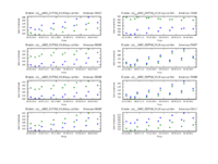
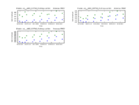
This mildly complicated sequence loops over all of our files and plots Tsys as a function of time for channel 1200 in spectral window 1. The subplot parameter sets up a 4 x 2 panel grid. Because this is not enough to show all antennas at once, there are two plotcal calls: one for the first 8 antennas (antenna=0~7) and one for any remaining antennas (antenna=8~15). The fontsize needs to be set to a small value or the text overlaps.
The 'raw_input' commands will wait for you hit hit Enter before issuing the next plot command. In the example above these are commented out (the leading "#" means that CASA will ignore them). If you would like to interactively cycle through the plots, uncomment them by removing the "#". Otherwise, the figfile parameter directs the output to .png files for later inspection. The easiest way to look at the 20 plots produced here is to simply inspect the .png files using your favorite viewer.
The Tsys values in Figure 2 look reliable, with typical values ~150 K except for some large values of Tsys at ~300 and 400 K for DV04. We will flag the data for that antenna.
We will also want to look at Tsys as a function of frequency. The following commands step through how you would do this, but do not execute this command blindly! (just in case, we have included a "break" that you will need to remove before running or the for loop will simply cancel).
#In CASA

for asdm in basename_all:
    break
    print "Plotting Tsys vs. frequency for "+asdm
    plotcal(caltable=asdm+'.tsys.cal.fdm',
	    xaxis="freq",yaxis="amp",
	    spw='1', plotsymbol=".", subplot=421,
	    iteration='antenna', figfile=asdm+'.tsys_vs_freq.page1.png',
	    antenna='0~7', fontsize=6.0)
    #dummy_string = raw_input("Inspecting Tsys table for "+asdm+" . Hit <Enter> to continue.")
    plotcal(caltable=asdm+'.tsys.cal.fdm',
	    xaxis="freq",yaxis="amp",
	    spw='1', plotsymbol=".", subplot=421,
	    iteration='antenna', figfile=asdm+'.tsys_vs_freq.page2.png',
	    antenna='8~15', fontsize=6.0)
    #dummy_string = raw_input("Inspecting Tsys table for "+asdm+" . Hit <Enter> to continue.")
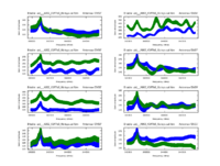
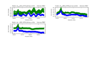
The commands are similar to the Tsys vs. time plotcal but will take much longer to run because instead of tracking a single channel we now plot the data for all 3840 channels in spw 1. Future enhancements to CASA will make it possible to plot these data more efficiently (e.g., by stepping across channels) but for now it takes a long time to generate these plots. We have included them in the directory "tsys_plots/" in the distribution you downloaded so that you will not need to generate them yourself. If you really want to run this command, remove the "break" and run the commands above.
Have a look at them now or see Figure 3 for an example on the first data set. You can a mesospheric absorption line at about 343.2 GHz that makes Tsys larger near that frequency in all antennas. Applying the Tsys calibration tables will minimize the contribution of these atmospheric lines. Again DV04 stands out with its very high Tsys.
We are now ready to apply the Tsys and the WVR calibration tables to the data with applycal. Again we loop through all the datasets. It is important to only apply Tsys and WVR corrections obtained close in time to the data being corrected, so in addition to looping over data sets we define the list of unique source names and loop over these. Then by setting gainfield and field to the same value we ensure that Tsys and WVR calibrations are only applied to the source for which they area measured. Because the source has a different name in the Northern Mosaic and the Southern Mosaic, we will carry out two loops.
# In CASA

basename_north=["uid___A002_X1ff7b0_Xb","uid___A002_X207fe4_X3a","uid___A002_X207fe4_X3b9","uid___A002_X2181fb_X49"]
field_names_north = ['Titan','3c279','NGC*']

for asdm in basename_north:
    print "Apply Tsys, WVR, and Antenna Position calibrations to "+asdm
    for field in field_names_north:
        applycal(vis=asdm+".ms", spw='1',
            field=field, gainfield=["",field,field],
            interp='nearest',
            gaintable=[asdm+".antpos",asdm+".tsys.cal.fdm",asdm+'.wvr.cal'],
            flagbackup=F)

basename_south=["uid___A002_X1ff7b0_X1c8","uid___A002_X207fe4_X1f7","uid___A002_X207fe4_X4d7",
                           "uid___A002_X215db8_X18","uid___A002_X215db8_X1d5","uid___A002_X215db8_X392"]
field_names_south = ['Titan','3c279','Ant*']

for asdm in basename_south:
    print "Apply Tsys and WVR calibrations to "+asdm
    for field in field_names_south:
        applycal(vis=asdm+".ms", spw='1',
            field=field, gainfield=["",field,field],
            interp='nearest',
            gaintable=[asdm+".antpos",asdm+".tsys.cal.fdm",asdm+'.wvr.cal'],
            flagbackup=F)
where:
- field: the field to which we will apply the calibration,
- gainfield: the field from which we wish to take the calibration table
- spw='1' : select only spectral window 1
- interp='nearest': use the interpolation mode to the 'nearest' solution.
As you browse through the whole data set, you will probably note some problems along the same lines as the DV04 issue we saw above. We'll apply these as additional data flagging in just a moment. First, with the Tsys and WVR calibrations applied successfully and the a priori flagging taken care of we will now split out the corrected data. We will keep only the corrected data, specified via 'datacolumn', and only spectral window 1, which contains the FDM (high spectral resolution) observations of the CO(3-2) line. We give the new MS files the extension ".wvrtsys.ms" to indicate that they have been corrected for WVR and Tsys effects. Because split will not overwrite existing files, we remove any previous versions of the new MS before beginning.
# In CASA
for asdm in basename_all:
    os.system('rm -rf '+asdm+'.wvrtsys.ms')
    print "Splitting out corrected data for "+asdm
    split(vis=asdm+'.ms', outputvis=asdm+'.wvrtsys.ms',
        datacolumn='corrected', spw='1')
The WVR and Tsys-corrected data now sit in the DATA column of the new measurement sets, which have only one spectral window (now labeled spectral window 0 though it was spectral window 1 in the original data). You may wish to run listobs to illustrate the changes:
# In CASA
for asdm in basename_all:
    listobs(vis=asdm+'.wvrtsys.ms', listfile=asdm+'.wvrtsys.listobs.txt', verbose=True)
Note the new spectral window information:
2011-08-05 01:07:08 INFO listobs	Spectral Windows:  (1 unique spectral windows and 1 unique polarization setups)
2011-08-05 01:07:08 INFO listobs	  SpwID  #Chans Frame Ch1(MHz)    ChanWid(kHz)TotBW(kHz)  Ref(MHz)    Corrs
2011-08-05 01:07:08 INFO listobs	  0        3840 TOPO  344845.586  488.28125   1875000     344908.33   XX  YY
Inspect and Flag Data
We are not quite done with the original ".ms" data sets yet. Before going further it will be useful to use plotms to show the effects of applying the calibration. In the process we'll take a quick look at each antenna and (hopefully) identify any pathologies in the data set.
For this basic inspection, we want to compare the phase and amplitude as a function of frequency and time in the DATA and CORRECTED columns of each measurement set. The CORRECTED column has had the Tsys and WVR calibrations applied and so we expect lower phase scatter and flatter amplitude response as a function of time and frequency. We are looking for antenna-based issues, so cycling through a set of baselines that includes each antenna once will be a good start. We'll focus these plots on the phase+bandpass calibrator, 3c279, and on baselines that include antenna DV11, which we will make our reference antenna in just a bit.
First, we plot amplitude as a function of frequency for 3c279. We start by plotting the DATA column, set color to indicate the two correlations (i.e., the XX and YY polarizations), and ask plotms to iterate over baseline. By setting antenna to 'DV11&*' we select only baselines that include DV11. We ask plotms to average all data over a very long timescale (timebin = 1e8 seconds ~ 3 years, much longer than the time for the whole data set) and allow it to average across scan boundaries by making avgscan = True. The result is a plot of average amplitude per channel vs. frequency.
# In CASA
basename_all=["uid___A002_X1ff7b0_Xb","uid___A002_X207fe4_X3a","uid___A002_X207fe4_X3b9",
     "uid___A002_X2181fb_X49","uid___A002_X1ff7b0_X1c8","uid___A002_X207fe4_X1f7",
     "uid___A002_X207fe4_X4d7","uid___A002_X215db8_X18","uid___A002_X215db8_X1d5",
     "uid___A002_X215db8_X392"]

asdm=basename_all[0]

plotms(vis=asdm+'.ms',
       field='3c279',
       xaxis='frequency', yaxis='amp',
       selectdata=T, spw='1',
       avgtime='1e8',avgscan=T,
       coloraxis='corr',
       iteraxis='baseline',
       antenna='DV11&*',
       ydatacolumn='data')
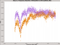
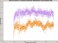
Notice the green arrows along the bottom of the plotms window. We asked plotms to iterate over baseline. As you click the arrows, the plot will rotate from baseline to baseline, always with DV11 so that each antenna shows up once. To see the effect of the calibration, go to the 'Axes' tab along the left of the plotms window and pull down the Data Column menu under the Y Axis. Set this from DATA to CORRECTED and you should see the effects of the calibration. You may need to ensure that the "Force Reload" box is checked before clicking "Plot" (both buttons lie at the bottom of the panel). For the most part things get better (flatter), but as we noted before DV04 is problematic.
You can now make analogous calls to example the phase vs. frequency, amplitude vs. time, and phase vs. time.
# In CASA

plotms(vis=asdm+'.ms',
       field='3c279',
       xaxis='frequency', yaxis='phase',
       selectdata=T, spw='1',
       avgtime='1e8',avgscan=T,
       coloraxis='corr',
       iteraxis='baseline',
       antenna='DV11&*',
       ydatacolumn='data')

plotms(vis=asdm+'.ms',
       field='3c279',
       xaxis='time', yaxis='amp',
       selectdata=T, spw='1:1200~1300',
       avgchannel='1000',avgscan=F,
       coloraxis='corr',
       iteraxis='baseline',
       antenna='DV11&*',
       ydatacolumn='data')

plotms(vis=asdm+'.ms',
       field='3c279',
       xaxis='time', yaxis='phase',
       selectdata=T, spw='1:1200~1300',
       avgchannel='100',avgscan=F,
       coloraxis='corr',
       iteraxis='baseline',
       antenna='DV11&*',
       ydatacolumn='data')
In each case, you will want to examine each baseline, alternating between the DATA and CORRECTED columns.
This is a lot of data inspection and that's only for one of 10 data sets! You can iterate across the data by hand, updating asdm to refer to each data set in order and cycling between baselines and DATA/CORRECTED by hand. It is also possible to script CASA to show you the key plots in succession (see the next block down). However you approach the infrastructure, you are looking for:
- Improved scatter and lower variability in phase and amplitude vs. frequency and time. This indicates that the WVR and Tsys calibrations helped.
- Sudden jumps in phase or amplitude as a function of either time or frequency. These may indicate problems with the antenna during the track.
- Large gradients (wrapping) in phase as a function of frequency. This may indicate a problem in the delays (signal path length to the telescope).
- Unusual magnitude, scatter, or patterns in any plot - though this may be better explored using plots that show all data together, which we'll make in a moment.
- Missing data. If the phase calibrator drops out for a period of time we will not be able to calibrate and will need to flag the data.
As you look through, note individual potentially problematic antennas. If all antennas in a data set appear problematic it may be that your "reference" (in the example above, DV11) is the source of the problem. In this case swap this reference antenna for another and see to the problem is isolated to DV11.
If you do wish to semi-automate the plot generation, the following sequence will cycle between data and corrected plots for each data set in turn. Type "stop" at any input call to break out.
# In CASA

for asdm in basename_all:

    # Extract antenna list for this data set.
    tb.open(asdm+'/ANTENNA', nomodify=True)
    ants = tb.getcol('NAME')
    tb.close

    # Define the reference antenna to make baselines with
    ref_ant = 'DV11'
    user_input = ""
    for ant in ants:

        if user_input == "stop":
            break

        # Skip correlation of reference antenna with itself (autocorrelations are flagged anyhow)
        if ant == ref_ant:
            continue

        ant_str = ref_ant+'&'+ant
        print "Showing baseline "+ant_str+" for data set "+asdm
        print "Use this inspect effect of applying wvrcal and Tsys calibrations."

        for y_axis in ["amp", "phase"]:

            print "... "+y_axis+" vs. frequency for DATA:"
            plotms(vis=asdm+'.ms', spw='1', field='3c279',
               antenna=ant_str, xaxis="frequency", yaxis=y_axis,
               avgtime="1e8", avgscan=T, coloraxis="corr",
               ydatacolumn="data")
            user_input = raw_input("Hit <ENTER> to see CORRECTED data [type 'stop'+<Enter> to break out].")
            if user_input == "stop":
                break

            print "... "+y_axis+" vs. frequency for CORRECTED:"
            plotms(vis=asdm+'.ms', spw='1', field='3c279',
               antenna=ant_str, xaxis="frequency", yaxis=y_axis,
               avgtime="1e8", avgscan=T, coloraxis="corr",
               ydatacolumn="corrected")
            user_input = raw_input("Hit <ENTER> to proceed to next plot [type 'stop'+<Enter> to break out].")
            if user_input == "stop":
                break

            print "... "+y_axis+" vs. time for DATA:"
            plotms(vis=asdm+'.ms', spw='1:1200~1300', field='3c279',
               antenna=ant_str, xaxis="time", yaxis=y_axis,
               avgchannel="1000", coloraxis="corr",
               ydatacolumn="data")
            user_input = raw_input("Hit <ENTER> to see CORRECTED data [type 'stop'+<Enter> to break out].")
            if user_input == "stop":
                break

            print "... "+y_axis+" vs. time for CORRECTED:"
            plotms(vis=asdm+'.ms', spw='1:1200~1300', field='3c279',
               antenna=ant_str, xaxis="time", yaxis=y_axis,
               acgchannel="1000", coloraxis="corr",
               ydatacolumn="corrected")
            user_input = raw_input("Hit <ENTER> to proceed to next plot [type 'stop'+<Enter> to break out].")
            if user_input == "stop":
                break
A detailed explanation of the procedure is a bit outside the scope of this guide, but the basic process is to loop over each data set, baseline with the reference antenna (here DV11), and y-axis of interest (phase or amplitude) then plot the effect of the calibration vs. frequency and time for each combination. Running this to step through the data will give you about 200 "before and after" plots from which you could note a subset of problematic cases to be followed up by hand. Many other strategies to inspect the data are also viable.
Next we will do a bit more inspection using plotms to look at whole data sets. This will help us identify missing data or look for egregious outliers.
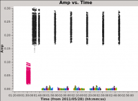
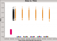
First we plot amplitude versus time (see Figure 5), averaging over all channels (by setting avgchannel to the very large value 10,000). We colorize by field so that scans on Titan are red, the bandpass and phase calibrator 3c279 is black (and orange in the Southern Mosaic where it has two field IDs), and the Antennae mosaic appears as a range of colors (one per pointing).
# In CASA
for asdm in basename_all:
    plotms(vis=asdm+'.wvrtsys.ms',
            xaxis='time', yaxis='amp',
            avgchannel='10000',coloraxis='field')
    dummy_string = raw_input("Examining amplitude vs. time for "+asdm+" . Hit <Enter> to proceed.")
Here look for:
- Missing data. The source needs to be flanked by phase calibrator scans, if those are missing for any reason we need to flag the appropriate time range.
- Dramatic outliers. Does the source suddenly get very bright or the otherwise bright calibrator appear anomalously faint for a brief time? This likely indicates problematic data that should be identified and flagged. You can use the 'select' (box with green plus) and 'locate' (magnifying glass) buttons in plotms to isolate and identify problem data (it will print to the log).
- Smooth variation with time. A sudden jump may indicate a problem and often the safest approach is to flag data near a discontinuity.
Look through the amplitudes vs. time for each data set (remember that we've already examined the phases vs. time and amplitude vs. time for individual baselines above).
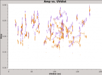
There are two other very useful "averaging" plots worth making. First, we plot amplitude as a function of u-v distance (projected antenna separation). Discontinuities and spikes in this plot are often from non-astrophysical sources. In the phase analog to the plot, the effects of atmospheric decorrelation can be assessed from increased scatter at longer u-v distances. While using the moon Titan as our flux calibrator, we may want to watch for flaring amplitudes at short u-v distances. These may indicate that Saturn is contaminating our beam. For a perfect, bright point source, we expect flat amplitudes as a function of u-v distance at the source amplitudes. Figure 6 shows an example of this plot, generated via:
# In CASA
for asdm in basename_all:
    plotms(vis=asdm+'.wvrtsys.ms',
        field='3c279',
        xaxis='uvdist', yaxis='amp',
        avgchannel='10000',coloraxis='corr')
    dummy_string = raw_input("Examining amplitude vs. time for "+asdm+" . Hit <Enter> to proceed.")
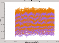
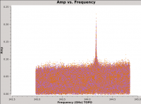
It can also be useful to examine the average amplitude as a function of frequency for each targets. This allows one to check for lingering atmospheric effects, unexpected line emission or absorption in the calibrators, or decreased sensitivity due to "roll-off" of the telescope sensitivity at the band edges.
# In CASA
field_names = ["3c279","Titan","NGC*","Ant*"]

for asdm in basename_all:
    for field in field_names:
        plotms(vis=asdm+'.wvrtsys.ms',
            field=field,
            xaxis='frequency', yaxis='amp',
            avgtime='1e8',avgscan=T, coloraxis='corr')
        dummy_string = raw_input("Examining amplitude vs. frequency for "+field+" in "+asdm+" . Hit <Enter> to proceed.")
This suite of plots (along with the earlier inspection of the Tsys tables) gives us the tools we need to identify problematic data through the data sets. We use this to generate a set of inspection-driven flagdata commands for each data set. We apply these before calibration.
This is the full set of flagging that we use for this data set. Your mileage may vary:
# In CASA

# First, flag the less sensitive edge channels of every data set
for asdm in basename_all:
    flagdata(vis = asdm+'.wvrtsys.ms',spw = '0:0~7,1:3831~3839', flagbackup = F)

### NORTHERN MOSAIC DATA SETS

### ... set 1
asdm="uid___A002_X1ff7b0_Xb"

# Problematic Tsys measurements
flagdata(vis=asdm+'.wvrtsys.ms', mode='manualflag',antenna='DV04', flagbackup = F)

flagmanager(vis=asdm+'.wvrtsys.ms',mode='save',versionname ='User')

### ... set 2
asdm="uid___A002_X207fe4_X3a"

# DV09 shows a phase jump. Flag near that time range.
flagdata(vis=asdm+'.wvrtsys.ms',mode='manualflag',antenna='DV09', timerange='21:24:09~21:35:35', flagbackup = F)

# The Tsys calibration had issues for one correlation in DV12, leading to spurious spikes toward low amplitude in several data set
flagdata(vis=asdm+'.wvrtsys.ms',antenna='DV12',spw='0:638~641;1663~1664;2430~2433',correlation='YY')

flagmanager(vis =asdm+'.wvrtsys.ms',mode = 'save',versionname = 'User')

### ... set 3
asdm="uid___A002_X207fe4_X3b9"

# the last calibrator (3c279) was not observed so we flag the last source scan
flagdata(vis=asdm+'.wvrtsys.ms',mode='manualflag',timerange='00:53:47~01:08:00',flagbackup = F)

# same DV12 issue
flagdata(vis=asdm+'.wvrtsysms',antenna='DV12',spw='0:638~641;1663~1664;2430~2433',correlation='YY',flagbackup=F)

flagmanager(vis=asdm+'.wvrtsys.ms',mode = 'save',versionname = 'User')

### ... set 4
asdm="uid___A002_X2181fb_X49"

# same DV12 issue
flagdata(vis=asdm+'.wvrtsys.ms',antenna='DV12',spw='0:638~641;1663~1664;2430~2433',correlation='YY',flagbackup=F)

flagmanager(vis=asdm+'.wvrtsys.ms',mode = 'save',versionname = 'User')

### SOUTHERN MOSAIC DATA SETS

### ... set 5

# the last calibrator (3c279) scan was not observed so we flag the last source scan.
flagdata(vis=asdm+'.wvrtsys.ms',mode='manualflag',antenna='DV10',timerange='19:46:20~20:34:40',flagbackup=F)

# DV13 shows evidence for some delay problems and large phase scatter
flagdata(vis=asdm+'.wvrtsys.ms',mode='manualflag',antenna='DV13',flagbackup=F)

flagmanager(vis =asdm+'.wvrtsys.ms',mode = 'save',versionname = 'User')

### ... set 6
asdm="uid___A002_X1ff7b0_X1c8"

# Problematic high Tsys values on DV04.
flagdata(vis=asdm+'.wvrtsys.ms',mode='manualflag',antenna='DV04',flagbackup=F)

flagmanager(vis=asdm+'.wvrtsys.ms',mode = 'save',versionname = 'User')

### ... set 7
asdm="uid___A002_X207fe4_X1f7"

flagdata(vis=asdm+'.wvrtsys.ms',mode='manualflag',antenna='DV09',timerange='23:30:52~24:10:00',flagbackup=F)

flagdata(vis=asdm+'.wvrtsys.ms',mode='manualflag',antenna='PM01',timerange='23:16:50~24:10:00',flagbackup=F)

flagdata(vis=asdm+'.wvrtsys.ms',mode='manualflag',antenna='PM03',timerange='23:16:50~24:10:00',flagbackup=F)

flagmanager(vis=asdm+'.wvrtsys.ms',mode = 'save',versionname = 'User')

### ... set 8
asdm="uid___A002_X207fe4_X4d7"

flagmanager(vis=asdm+'.wvrtsys.ms',mode='save',versionname='User')

### ... set 9
asdm="uid___A002_X215db8_X1d5"

# same DV13 issue
flagdata(vis=asdm+'.wvrtsys.ms',mode='manualflag',antenna='DV13',flagbackup=F)

# same DV12 issue
flagdata(vis=asdm+'.wvrtsys.ms',antenna='DV12',spw='0:638~641;1663~1664;2430~2433',correlation='YY',flagbackup=F)

flagmanager(vis=asdm+'.wvrtsys.ms',mode = 'save',versionname = 'User')

### ... set 10
asdm="uid___A002_X215db8_X392"

# same DV13 issue
flagdata(vis=asdm+'.wvrtsys.ms',mode='manualflag',antenna='DV13',flagbackup=F)

flagmanager(vis=asdm+'.wvrtsys.ms',mode = 'save',versionname = 'User')
Applying this flagging will remove the most egregious outliers. We are now ready to calibrate the data.
Bandpass Calibration
We begin by calibrating the phase and amplitude response of each antenna as a function of frequency, called "bandpass calibration." We have already seen that the data contain smooth but systematic variations in both phase and amplitude as a function of frequency. We can see this again in a more compact form by plotting
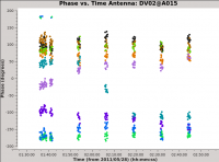
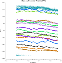
Next we plot the phase as a function of time and frequency for the bandpass calibrator, 3c279. For the first plot, Figure 7, we use avgscan=T and avgtime='1e8' to average in time over all scans and integrations, and we specify coloraxis='baseline' to colorize by baseline. For the second, Figure 8, we use spw='0:40~3800' and avgchannel='3840' to average over the central channels of the first spectral window. For both plots we will iterate on antenna (interaxis='antenna'). Use the green arrows of the plotms GUI to view the plots for different antennas.
# In CASA

plotms(vis= asdm+'.split.ms',
            xaxis='freq', yaxis='phase',
            selectdata=True, field='3c279', corr='XX', antenna='*&*',
            avgtime='1e8', avgscan=T,
            coloraxis='baseline', iteraxis='antenna')
# In CASA

plotms(vis= asdm+'.split.ms',
           xaxis='time', yaxis='phase',
           selectdata=True, field='3c279',
           spw='0:40~3800', antenna='*&*',corr='XX',
           avgchannel='3840',  avgscan=T,
           coloraxis='baseline', iteraxis='antenna')
Figure 7 shows that the phase varies with time, thus it will need to be gain calibrated. In Figure 8 we see that phase variations as a function of frequency in dataset uid_A002_X1ff7b0_Xb are small, typically ~ 30 degrees, thus bandpass calibration will suffice (i.e. no delay calibration is needed).
We issue gaincal on 3c279 to determine phase(-only) gain solutions. We use solint='int' for the solution interval, which means that one gain solution will be determined for every integration time to prevent de-correlation of the signal. Once phase is corrected, we can determine the bandpass solutions with bandpass. We apply the phase calibration table on-the-fly with the parameter "gaintable". Bandpass response can vary from day to day, therefore we calculate independent bandpass solutions for each dataset.
#In CASA

for asdm in basename_all:
  os.system('rm -rf '+asdm+'.bpphase.gcal,'+asdm+'.bandpass.bcal')
  gaincal(vis = asdm+'.split.ms',
               selectdata=T,field = '3c279',spw = '0:40~3800',
               caltable = asdm+'.bpphase.gcal',
               solint = 'int',refant = 'DV09',calmode='p')
  bandpass(vis = asdm+'.split.ms',
               field = '3c279',
               gaintable = asdm+'.bpphase.gcal',
               caltable = asdm+'.bandpass.bcal',
               bandtype='B',
               solint = 'inf',combine = 'scan', solnorm=T,refant = 'DV09',
               minblperant=3,minsnr=2,fillgaps=1)
where:
- gaintable = asdm+'.bpphase.gcal', caltable = asdm+'.b1.cal': Gain calibration table, and bandpass calibration table
- solint='int' or 'inf': The former is to consider integration by integration. The latter, combined with the default combine='scan', sets the solution interval to the entire observation
- refant = 'DV09': Set the reference antenna to DV06
- calmode='p': Gain cal calibration only phase
- minblperant=3: Minimum number of baselines required per antenna for each solve
- minsnr=2: Minimum SNR for solutions
- bandtype='B': Channel by channel solution for each specified spw
- fillgaps=1: Interpolate channel gaps 1 channel wide
- solnorm=T: Normalize the bandpass amplitudes and phases of the corrections to unity
Do not worry about the message "Insufficient unflagged antennas" when running the bandpass task, which relates to the flagged edge channels.
We plot the time variation of the phase solutions (asdm+'.bpphase.gcal') using plotcal, to check that they vary smoothly with time.
#In CASA
  plotcal(caltable = asdm+'.bpphase.gcal',
              xaxis = 'time',yaxis = 'phase',
              iteration = 'antenna',plotrange=[0,0,-180,180])
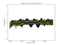
We also plot the bandpass solutions with plotcal, and we see that the solutions seem reasonable, with amplitudes close to 1 (Figure 9), and phases that does not vary much over the spectral window.
#In CASA
  plotcal(caltable = asdm+'.bandpass.bcal',
              xaxis = 'freq',yaxis = 'amp',
              plotrange = [0,0,0.8,1.2])

  plotcal(caltable = asdm+'.bandpass.bcal',
              xaxis = 'freq',yaxis = 'phase',
              plotrange = [0,0,-100,100])
Gain (Phase and Amplitude) Calibration
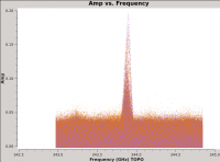
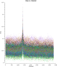
We set the flux for our flux calibrator, Titan, using the task setjy, by applying the Butler-JPL-Horizons 2010 model. First, we check the flux calibrator data. We plot the spectrum and find a bright line emission (Figure 10) in the spectral window. We will flag it using flagdata and update the flag version using flagmanager.
# in CASA
for asdm in basename_all:
  flagdata(vis=asdm+'.split.ms',flagbackup=F,
         field=['Titan'],
         spw=['0:1100~1700'])
  flagmanager(vis =asdm+'.split.ms',mode = 'save',versionname = 'FlagFlux')
Second, we do a new gain calibration applying the bandpass calibration solutions on-the-fly.
We solve for amplitude and phase simultaneously and determine average solutions per scan.
# in CASA
for asdm in basename_all:
  os.system('rm -rf '+asdm+'.amp.gcal,'+asdm+'.flux.cal')
  setjy(vis = asdm+'.split.ms',field = 'Titan',
           standard = 'Butler-JPL-Horizons 2010')

  gaincal(vis=asdm+'.split.ms',
                gaintable=asdm+'.bandpass.bcal',
                caltable=asdm+'.intphase.gcal',
                calmode='p',
                field='Titan,3c279',
                spw='0~1:40~3800',
                refant='DV09', solint='int',minsnr=2.0,minblperant=4)

  gaincal(vis=asdm+'.split.ms',
                gaintable=asdm+'.bandpass.bcal',
                caltable=asdm+'.scanphase.gcal',
                calmode='p',
                field='Titan,3c279',
                spw='0~1:40~3800',
                refant='DV09', solint='inf',minsnr=2.0,minblperant=4)

  gaincal(vis = asdm+'.split.ms',
               gaintable =[asdm+'.bandpass.bcal',asdm+'.intphase.gcal'],
               caltable = asdm+'.amp.cal',
               calmode='ap'
               field = 'Titan, 3c279',
               refant = 'DV09',solint = 'int')
Finally, we will bootstrap the flux density of the secondary calibrator from that of Titan using the task fluxscale.
# in CASA
  fluxscale(vis = asdm+'.split.ms',
                 caltable = asdm+'.amp.gcal',
                 fluxtable = asdm+'.flux.cal',
                 reference = 'Titan',
                 transfer = '3c279')
The flux of Titan at these frequencies is about 2.9 Jy. For example, for dataset uid___A002_X1ff7b0_Xb.f1.cal:
#2011-07-13 07:31:04 INFO setjy Titan spwid= 0 [I=2.846, Q=0, U=0, V=0] Jy
The new flux table asdm+'.flux.gcal' replaces the previous asdm+'.amp.gcal table in future application of the calibration to the data, i.e. the new flux table contains both asdm+'.amp.gcal and the newly acquired flux scaling. Unlike the gain calibration steps, this is not an incremental table.
- gaintable = asdm+'.bandpass.bcal': We apply the bandpass calibration on-the-fly
- caltable = 'asdm+'.amp.cal: the output gain calibration table
- calmode = 'ap': To solve for amplitude and phase
We find that the flux of 3c279 is 10.45 Jy, by averaging the fluxes obtained from the ten available datasets. This flux agree within 10% with the most recent 0.850 mm measurements from the SMA calibrator list [1] : (01 Jul 2011, SMA 9.75 ± 0.49).
Apply the Calibrations and Inspect
Now we will use applycal to apply the bandpass, phase, and amplitude calibration tables that we generated in the previous sections to the data. We apply the solutions separately to the bandpass and secondary ("phase") calibrator 3c279, the flux calibrator Titan, and the source. In most data sets the bandpass and secondary calibrator will not be the same and this step would include one additional applycal.
#In CASA
basename_all=["uid___A002_X1ff7b0_Xb","uid___A002_X207fe4_X3a","uid___A002_X207fe4_X3b9",
     "uid___A002_X2181fb_X49","uid___A002_X1ff7b0_X1c8","uid___A002_X207fe4_X1f7",
     "uid___A002_X207fe4_X4d7","uid___A002_X215db8_X18","uid___A002_X215db8_X1d5",
     "uid___A002_X215db8_X392"]

for asdm in basename_all:
  applycal(vis=asdm+'.split.ms',field='3c279',
        gaintable=[asdm+'bandpass.bcal',asdm+'.intphase.gcal',asdm+'.flux.cal'],
        interp=['nearest','nearest','nearest'],
        gainfield=['3c279','3c279','3c279'],flagbackup=T)

  applycal(vis=asdm+'.split.ms',field='Titan',
        gaintable=[asdm+'bandpass.bcal',asdm+'.intphase.gcal',asdm+'.flux.cal'],
        interp=['nearest','nearest','nearest'],
         gainfield=['3c279','Titan','Titan'],flagbackup=T)

  applycal(vis=asdm+'.split.ms',field=['Ant*','NGC*']
        interp=['nearest','linear','linear'],
        gaintable=[asdm+'bandpass.bcal',asdm+'.scanphase.gcal',asdm+'.flux.cal'],
        gainfield=['3c279','3c279','3c279'],flagbackup=T)
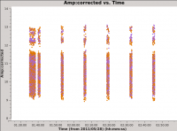
We plot the corrected amplitudes and phases of 3c279 as a function of time and frequency, to check that the phases are close to zero and the amplitudes are constant.
# In CASA
asdm=basename_all[0]
plotms(vis = asdm+'.split.ms', xaxis='time', yaxis='amp',
	ydatacolumn='corrected', selectdata=True, field='3c279',
	averagedata=True, avgchannel='3840', avgtime='',
	avgscan=F, avgbaseline=F, coloraxis='spw')

plotms(vis = asdm+'.split.ms', xaxis='time', yaxis='pha',
	ydatacolumn='corrected', selectdata=True, field='3c279',
	averagedata=True, avgchannel='3840', avgtime='',
	avgscan=F, avgbaseline=F, coloraxis='spw')

plotms(vis = asdm+'.split.ms', xaxis='time', yaxis='pha',
	ydatacolumn='corrected', selectdata=True, field='3c279',
	averagedata=True, avgchannel='', avgtime='1e6',
	avgscan=T, avgbaseline=F, coloraxis='baseline')

plotms(vis = asdm+'.split.ms', xaxis='time', yaxis='pha',
	ydatacolumn='corrected', selectdata=True, field='3c279',
	averagedata=True, avgchannel='', avgtime='1e6',
	avgscan=T, avgbaseline=F, coloraxis='baseline')
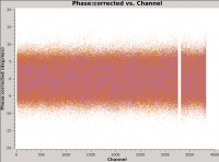
In Fig. 11 and 12 we plot phase vs. channel and amp vs. time for 3c279 for the uid___A002_X1ff7b0_Xb dataset.
Finally we can use plotms to examine the corrected amplitude and phase of Antennae galaxies as a function of frequency, just by changing the field keyword to field='NGC*','Antennae*'.
Split and Concatenate Data for Northern and Southern Mosaics
The individual data sets are now calibrated. We can safely split out the calibrated data for our science target and drop the calibrators. As we do so, we will smooth the data in frequency by setting, averaging together groups of 10 channels by setting width=10 in split. The new data will have a channel width corresponding to about ~4.5 km/s. This will make the imaging steps much more tractable.
#In CASA

basename_all=["uid___A002_X1ff7b0_Xb","uid___A002_X207fe4_X3a","uid___A002_X207fe4_X3b9",
     "uid___A002_X2181fb_X49","uid___A002_X1ff7b0_X1c8","uid___A002_X207fe4_X1f7",
     "uid___A002_X207fe4_X4d7","uid___A002_X215db8_X18","uid___A002_X215db8_X1d5",
     "uid___A002_X215db8_X392"]

for asdm in basename_all:
    os.system('rm -rf '+asdm+'.cal.ms')
    split(vis = asdm+'.wvrtsys.ms',outputvis = asdm+'.cal.ms',
             field = ['NGC*','Antennae*'],spw='0',width=10)
    listobs(asdm+'.cal.ms',listfile=asdm+'.cal.listobs.txt')
For convenience we concatenate all data for the Northern Mosaic into a single big MS and place all data for the Southern Mosaic into another file. To do this, we construct a list that holds the names of all the Southern Mosaic MS files and another that holds the name of all the Northern Mosaic MS files then feed these into the concat task.
# In CASA
basename_north=["uid___A002_X1ff7b0_Xb","uid___A002_X207fe4_X3a","uid___A002_X207fe4_X3b9","uid___A002_X2181fb_X49"]

basename_south=["uid___A002_X1ff7b0_X1c8","uid___A002_X207fe4_X1f7","uid___A002_X207fe4_X4d7",
                           "uid___A002_X215db8_X18","uid___A002_X215db8_X1d5","uid___A002_X215db8_X392"]

cal_south_vis = [vis+'.cal.ms' for vis in basename_south]
cal_north_vis = [vis+'.cal.ms' for vis in basename_north]

os.system('rm -rf Antennae_South.cal.ms')
concat(vis=cal_south_vis, concatvis='Antennae_South.cal.ms', timesort=T)

os.system('rm -rf Antennae_North.cal.ms')
concat(vis=cal_north_vis, concatvis='Antennae_North.cal.ms', timesort=T)
The syntax used to construct the 'cal_south_vis' variable loops over basename_south and makes a list after adding '.cal.ms' to each member. To see the list 'print cal_south_vis'.
Continue on to Imaging of the Science Target
Now you can continue on to the imaging guide.
Daniel Espada 12:00 UT, 27 July 2011
