3C286 Band6Pol Calibration for CASA 5.7
Overview
This portion of the 3C286_Polarization CASA Guide will cover the calibration of the raw visibility data. To follow this guide you must have downloaded the file 3C286_Band6_UncalibratedData.tgz from 3C286_Polarization#Obtaining the Data.
Details of the ALMA observations are provided at 3C286_Polarization.
To skip to the imaging portion of the guide, see: 3C286_Band6Pol_Imaging.
This guide is designed for CASA 5.7.
Note that the calibration procedure described here is intended to provide an initial example of the reduction of ALMA polarization data. It may be updated in future, and is not necessarily the exact procedure by which Early Science data will be calibrated. A future Science Verification (SV) dataset on 3C 138 will demonstrate an updated calibration strategy. Details of the 3C 138 SV data can be found on the Science Verification webpage
Unpack the Data
Once the file 3C286_Band6_UncalibratedData.tgz has been download, unpack it as follows:
# in bash
# In a terminal outside CASA
tar -xvzf 3C286_Band6_UncalibratedData.tgz

cd 3C286_Band6_UncalibratedData


# Start CASA
casa
Confirm your version of CASA
This guide has been written for CASA release 5.7. Please confirm your version before proceeding.
# In CASA
import casadef
version = casadef.casa_version
print "You are using " + version
if (version < '5.7.0'):
    print "YOUR VERSION OF CASA IS TOO OLD FOR THIS GUIDE."
    print "PLEASE UPDATE IT BEFORE PROCEEDING."
else:
    print "Your version of CASA is appropriate for this guide."
We need to import some scripts we will use during the calibration
# In CASA
from recipes.almahelpers import fixsyscaltimes
path=os.getenv("CASAPATH").split(' ')[0]
execfile(path+'/lib/python2.7/recipes/almahelpers.py')
execfile(path+'/lib/python2.7/recipes/almapolhelpers.py')
Initial Inspection, A priori calibration
We will eventually concatenate the three datasets into one dataset. However, we will keep them separate for now, as some of the steps to follow require individual datasets (specifically, the application of the Tsys and WVR tables). We therefore start by defining an array "basename" that includes the names of the three files in chronological order. This will simplify the following steps by allowing us to loop through the files using a simple for-loop in python. Remember that if you log out of CASA, you will have to re-issue this command.
# In CASA
# Define a python list holding the names of all of our data sets
basename=["uid___A002_X85c183_X10a","uid___A002_X85c183_X51a", "uid___A002_X85c183_X822"]
The raw data have been provided to you in the ASDM format. It is the native format of the data produced by the observatory.
Before we can proceed to the calibration, we will need to convert those data to the CASA MS format. This is done simply with the task importasdm.
#In CASA
for name in basename:
        importasdm(asdm = name, asis='*')
The usual first step is then to get some basic information about the data. We do this using the task listobs, which will output a detailed summary of each dataset supplied.
# In CASA
# Loop over each element in the list and create summary file using listobs

for name in basename:
    os.system('rm '+name+'.listobs.txt')
    listobs(vis=name+'.ms', listfile=name+'.listobs.txt', verbose=True)
Note that after cutting and pasting a for-loop you often have to press return several times to execute. The output will be sent to the CASA logger, or saved in a text file. Here is a snippet extracted from the full verbose listobs output for the first file in the list:
Fields: 5
  ID   Code Name                RA               Decl           Epoch   SrcId      nRows
  0    none J1337-1257          13:37:39.782784 -12.57.24.69312 J2000   0        3400886
  1    none J1256-0547          12:56:11.166560 -05.47.21.52458 J2000   1         636058
  2    none Ceres               13:29:06.769601 -01.11.10.65438 J2000   2         546034
  3    none J1310+3220          13:10:28.663200 +32.20.43.80000 J2000   3         840937
  4    none 3c286               13:31:08.288100 +30.30.32.96000 J2000   4        4701150
Spectral Windows:  (25 unique spectral windows and 3 unique polarization setups)
  SpwID  Name                           #Chans   Frame   Ch0(MHz)  ChanWid(kHz)  TotBW(kHz) CtrFreq(MHz) BBC Num  Corrs
  0      WVR#NOMINAL                         4   TOPO  184550.000   1500000.000   7500000.0 187550.0000        0  XX
  1      ALMA_RB_06#BB_1#SW-01#FULL_RES    128   TOPO  215242.188    -15625.000   2000000.0 214250.0000        1  XX  YY
  2      ALMA_RB_06#BB_1#SW-01#CH_AVG        1   TOPO  214234.375   1796875.000   1796875.0 214234.3750        1  XX  YY
  3      ALMA_RB_06#BB_2#SW-01#FULL_RES    128   TOPO  217242.188    -15625.000   2000000.0 216250.0000        2  XX  YY
  4      ALMA_RB_06#BB_2#SW-01#CH_AVG        1   TOPO  216234.375   1796875.000   1796875.0 216234.3750        2  XX  YY
  5      ALMA_RB_06#BB_3#SW-01#FULL_RES    128   TOPO  229257.813     15625.000   2000000.0 230250.0000        3  XX  YY
  6      ALMA_RB_06#BB_3#SW-01#CH_AVG        1   TOPO  230234.375   1796875.000   1796875.0 230234.3750        3  XX  YY
  7      ALMA_RB_06#BB_4#SW-01#FULL_RES    128   TOPO  231257.813     15625.000   2000000.0 232250.0000        4  XX  YY
  8      ALMA_RB_06#BB_4#SW-01#CH_AVG        1   TOPO  232234.375   1796875.000   1796875.0 232234.3750        4  XX  YY
  9      ALMA_RB_06#BB_1#SW-01#FULL_RES    128   TOPO  224992.188    -15625.000   2000000.0 224000.0000        1  XX  YY
  10     ALMA_RB_06#BB_1#SW-01#CH_AVG        1   TOPO  223976.562   1781250.000   1781250.0 223976.5625        1  XX  YY
  11     ALMA_RB_06#BB_2#SW-01#FULL_RES    128   TOPO  226992.188    -15625.000   2000000.0 226000.0000        2  XX  YY
  12     ALMA_RB_06#BB_2#SW-01#CH_AVG        1   TOPO  225976.562   1781250.000   1781250.0 225976.5625        2  XX  YY
  13     ALMA_RB_06#BB_3#SW-01#FULL_RES    128   TOPO  239007.813     15625.000   2000000.0 240000.0000        3  XX  YY
  14     ALMA_RB_06#BB_3#SW-01#CH_AVG        1   TOPO  239976.563   1781250.000   1781250.0 239976.5625        3  XX  YY
  15     ALMA_RB_06#BB_4#SW-01#FULL_RES    128   TOPO  241007.813     15625.000   2000000.0 242000.0000        4  XX  YY
  16     ALMA_RB_06#BB_4#SW-01#CH_AVG        1   TOPO  241976.563   1781250.000   1781250.0 241976.5625        4  XX  YY
  17     ALMA_RB_06#BB_1#SW-01#FULL_RES     64   TOPO  224984.375    -31250.000   2000000.0 224000.0000        1  XX  XY  YX  YY
  18     ALMA_RB_06#BB_1#SW-01#CH_AVG        1   TOPO  223968.750   1781250.000   1781250.0 223968.7500        1  XX  XY  YX  YY
  19     ALMA_RB_06#BB_2#SW-01#FULL_RES     64   TOPO  226984.375    -31250.000   2000000.0 226000.0000        2  XX  XY  YX  YY
  20     ALMA_RB_06#BB_2#SW-01#CH_AVG        1   TOPO  225968.750   1781250.000   1781250.0 225968.7500        2  XX  XY  YX  YY
  21     ALMA_RB_06#BB_3#SW-01#FULL_RES     64   TOPO  239015.625     31250.000   2000000.0 240000.0000        3  XX  XY  YX  YY
  22     ALMA_RB_06#BB_3#SW-01#CH_AVG        1   TOPO  239968.750   1781250.000   1781250.0 239968.7500        3  XX  XY  YX  YY
  23     ALMA_RB_06#BB_4#SW-01#FULL_RES     64   TOPO  241015.625     31250.000   2000000.0 242000.0000        4  XX  XY  YX  YY
  24     ALMA_RB_06#BB_4#SW-01#CH_AVG        1   TOPO  241968.750   1781250.000   1781250.0 241968.7500        4  XX  XY  YX  YY
[...]
Antennas: 31:
  ID   Name  Station   Diam.    Long.         Lat.                Offset from array center (m)                ITRF Geocentric coordinates (m)
                                                                     East         North     Elevation               x               y               z
  0    DA41  A079      12.0 m   -067.45.13.6  -22.53.35.0        116.8369     -920.2897       22.6287  2225122.700426 -5439951.133460 -2481886.481390
  1    DA42  A081      12.0 m   -067.45.23.9  -22.53.32.5       -174.5620     -842.8378       21.0900  2224863.872997 -5440088.015712 -2481814.531125
  2    DA43  A091      12.0 m   -067.45.28.7  -22.53.24.2       -312.9125     -584.7726       23.7306  2224774.741865 -5440235.548469 -2481577.816103
  3    DA44  A068      12.0 m   -067.45.20.6  -22.53.25.7        -82.4244     -631.7829       23.5830  2224981.097391 -5440131.252519 -2481621.067210
  4    DA45  A070      12.0 m   -067.45.11.9  -22.53.29.3        166.1822     -743.4936       19.8824  2225193.449573 -5439993.765650 -2481722.541223
  5    DA46  A058      12.0 m   -067.45.17.3  -22.53.32.0         12.7400     -827.0339       21.9689  2225039.860423 -5440023.554679 -2481800.313874
  6    DA47  A074      12.0 m   -067.45.12.1  -22.53.32.0        161.8144     -828.6212       19.2711  2225176.657096 -5439964.248716 -2481800.726738
  7    DA48  A046      12.0 m   -067.45.17.0  -22.53.29.3         21.4254     -742.7993       21.6766  2225060.201673 -5440050.345525 -2481722.599573
  8    DA49  A029      12.0 m   -067.45.18.2  -22.53.25.8        -12.9141     -636.4555       22.1366  2225044.239474 -5440102.024044 -2481624.809292
  9    DA51  A082      12.0 m   -067.45.08.3  -22.53.29.2        269.0424     -740.9548       16.2831  2225287.766879 -5439952.669219 -2481718.802316
  10   DA54  A063      12.0 m   -067.45.16.1  -22.53.31.9         46.5810     -823.6376       21.9794  2225071.684905 -5440011.975810 -2481797.189115
  11   DA55  A080      12.0 m   -067.45.14.7  -22.53.20.2         87.4828     -461.2364       21.1332  2225162.612020 -5440126.242512 -2481462.996898
  12   DA56  A064      12.0 m   -067.45.14.7  -22.53.31.4         85.6567     -808.0287       21.5198  2225109.988756 -5440002.411268 -2481782.630797
  13   DA57  A076      12.0 m   -067.45.20.5  -22.53.33.8        -77.9911     -882.7200       24.5713  2224948.593535 -5440040.069448 -2481852.626444
  14   DA59  A021      12.0 m   -067.45.17.2  -22.53.27.0         14.3185     -672.8117       21.8450  2225063.988913 -5440078.377183 -2481658.189073
  15   DA62  A016      12.0 m   -067.45.16.4  -22.53.25.1         37.4652     -614.5612       21.7854  2225093.968954 -5440090.535537 -2481604.502426
  16   DV01  A072      12.0 m   -067.45.12.6  -22.53.24.0        147.1726     -580.5878       18.1840  2225199.253543 -5440058.163697 -2481571.803410
  17   DV02  A087      12.0 m   -067.45.08.3  -22.53.33.2        269.0953     -864.0700       16.2406  2225269.668853 -5439908.286857 -2481832.204625
[...]
This output shows that five fields were observed: J1337-1257, J1256-0547=3C279, Ceres, J1310+3220, and 3c286. The final column of the listobs output gives the scan intent. This information is used later to flag the pointing scans and the hot and ambient load calibration scans, using scan intent as a selection option. These intents are also used for pipeline processing. Field 0 (J1337-1257) will serve as the polarization calibrator; field 1 (3c279) as bandpass calibrator; field 2 (Ceres) will serve as the flux calibrator; field 3 (J1310+3220) as phase calibrator; and 3c286 (field 4) is, of course, the science target.
Spectral windows are marked with ID numbers from 0 to 24. If you look at one of the listobs.txt files, you may notice that there are additional SpwIDs listed in the "Sources" section that are not listed in the "Spectral Windows" section (this is not shown in the snippet above). These spws (15-62) are related to WVR measurements for each antenna, so you will not need them for the calibration either.
Spectral window 0 contains the WVR data; spws 1 to 16 also contain calibration data. The Tsys information is stored in spws 9, 11, 13, 15. In the listobs output shown above, you notice that field 3 (J1310+3220) has no Tsys measurements, since it is missing spws 9 to 16 in the spwIds. To increase observation efficiency, Tsys measurements are usually done either on the phase calibrator or the target. In the application of Tsys tables, we will apply to sources missing direct Tsys measurements the closest measurements available (see below).
The full polarization data are in spectral windows 17,19,21,23, which have 64 channels each. The channel width is 31.250 MHz and the total bandwidth is 2 GHz. There are two spws (17 and 19) in the lower sideband (LSB), centered at 224.984 and 226.984 GHz, respectively; and two spectral windows (spw 21 and 23) in the upper sideband (USB), centered at 239.015 and 241.015, respectively. Spectral windows 18,20,22,24 contain channel averages of the data in spectral windows 17,19,21,23, respectively. These are not useful for the offline data reduction.
Thirty-eight antennas were used for the dataset listed above. Note that numbering in python always begins with "0", so the antennas have IDs 0-37. To see what the antenna configuration looked like at the time of this observation, we use the task plotants.

# In CASA
plotants(vis=basename[0]+'.ms', figfile=basename[0]+'_plotants.png')
This will plot the antenna configuration on your screen (see Figure 1) as well as save it under the specified filename for future reference. We need to choose a reference antenna that is close to the center of the array (and is also stable and present for the entire observation). We will use antenna DV23 as reference antenna, and we define a variable to be used in the following tasks:
# In CASA
refant='DV23'
The other two datasets ("uid___A002_X85c183_X51a", "uid___A002_X85c183_X822") have been observed after "uid___A002_X85c183_X10a". From their listobs output we can see that, in both datasets, Ceres was not observed, and the field J1310+3220 does not have Tsys measurements.
Flagging
The first editing we will do is some a priori flagging with flagdata. ALMA data contain both the cross correlation and autocorrelation data, but here we are only interested in the cross-correlation data.
Now we will loop over the datasets, running these flagging commands:
# In CASA
for name in basename:
    flagdata(vis=name+'.ms',mode='manual', autocorr=True, flagbackup=False)
Some scans in the data were used by the online system for pointing and sideband ratio calibration. These scans are no longer needed, and we can flag them easily with flagdata by selecting on 'intent'. Similarly, we can flag the scans corresponding to atmospheric calibration since we no longer need them:
# In CASA
for name in basename:
    flagdata(vis=name+'.ms',mode='manual',
        intent='*POINTING*,*SIDEBAND_RATIO*,*ATMOSPHERE*', flagbackup=False)
We also flag "shadowed" data where one antenna blocks the line of sight of another.
# In CASA
for name in basename:
    flagdata(vis=name+'.ms',mode='shadow',flagbackup=False)
We will then store the current flagging state for each dataset using the flagmanager:
# In CASA
for name in basename:
    flagmanager(vis=name+'.ms', mode='save', versionname='Apriori')
See the Antennae casaguide (click here) for details on flagmanager.
Tsys and WVR calibration table generation
It turns out that two execution blocks (uid://A002/X85c183/X10a and X51a) out of the three taken on 2014-07-01 were affected by an ASDM SYSCal table issue. As a result, the Tsys values were incorrect and an entire scan is unintentionally flagged after applying the Tsys table. We need to run fixsyscaltimes task on these datasets before making the Tsys table.
# In CASA
fixsyscaltimes("uid___A002_X85c183_X10a.ms")
fixsyscaltimes("uid___A002_X85c183_X51a.ms")
fixsyscaltimes("uid___A002_X85c183_X822.ms")
We will loop over the datasets, generating the System Temperature (Tsys) and Water Vapour Radiometer (WVR) calibration tables for each of them.
The Tsys calibration gives a first-order correction for the atmospheric opacity as a function of time and frequency, and associates weights with each visibility that persist through imaging. Each ms file contains Tsys measurements; the task gencal is used to generate calibration tables from these measurements.
# In CASA
for name in basename:
    gencal(vis = name+'.ms',
        caltable = name+'.ms.tsys',
        caltype = 'tsys')
There are different ways to inspect Tsys calibration tables, in order to identify possibly wrong antenna solutions, see the TWhydraBand7 casaguide (click here) for details.
Here we use plotms to interactively plot Tsys vs frequency for all antennas.


# In CASA
plotms(vis=basename[0]+'.ms.tsys', xaxis='freq', yaxis='tsys', spw='',iteraxis='antenna',coloraxis='scan',showgui=True)
By using the next button it is possible to see the plots for each antenna. You will notice that all antennas have more or less the same behavior as antenna DA49 shown in Figure 2. Antenna DV21 clearly shows higher value of Tsys (see Figure 3), we will flag that antenna later in the combined dataset.
The plots look acceptable, aside from the large amplitudes in the edge channels. We flag the first four channels of each spw from the calibration tables.
# In CASA
for name in basename:
    flagdata(vis = name+'.ms.tsys',
             spw='9:0~3, 11:0~3, 13:0~3, 15:0~3')
To create the WVR calibration tables
we run the task wvrgcal. This task
examines the data for each ms as a whole and creates a calibration
table containing only phase corrections for each antenna and spw.
# In CASA
for name in basename:
    mylogfile = casalog.logfile()
    casalog.setlogfile(name+'.ms.wvrgcal')
    wvrgcal(vis = name+'.ms',
            caltable = name+'.ms.wvr',
            toffset = 0,
            tie = ['3c286,J1310+3220'],
            statsource = 'J1256-0547',
            wvrflag=['DA54'])
    casalog.setlogfile(mylogfile)
- casalog.setlogfile(mylogfile): we used this method to send the log output back to the original CASA log file.
WVR Correction and Tsys Calibration
We will now apply the Tsys and the WVR calibration tables to the data with the task applycal, which reads the specified gain calibration tables, applies them to the (raw) data column, and writes the calibrated results into the corrected column.
It is important to only apply Tsys and WVR corrections obtained close in time to the data being corrected.
In addition to looping over data sets, we can define the list of unique source names and loop over these. We set field and gainfield to ensure that the appropriate Tsys and WVR calibrations applied to each field. For J1337-1257, J1256-0547, and 3c286, this means using calibration obtained specifically on each of these fields; for J1310+3220, the Tsys from 3c286 is used. We will only correct spw 17,19,21,23, our science windows, because we will drop the other data in a moment.
We also need to tell applycal to use the Tsys information in spectral windows 9,11,13,15 for spectral window 17,19,21,23, respectively. We do so by specifying a list of spws. Normally we would use the almahelper function tsysspwmap (see here for details); however, in this case it gives a wrong result so we just define this list by hand:
# In CASA
tsysmap = [0,1,2,3,4,5,6,7,8,9,9,11,11,13,13,15,15,9,9,11,11,13,13,15,15]
Here we cycle over all datasets and fields (except Ceres):
# In CASA
field_names = ['J1337-1257','J1256-0547','3c286']
for name in basename:
    # General calibrators that have their own Tsys
    for field_name in field_names:
        applycal(vis = name+'.ms',
                 field = field_name,
                 spw = '17,19,21,23',
                 gaintable = [name+'.ms.tsys',name+'.ms.wvr'],
                 gainfield = [field_name,field_name],
                 interp = 'linear',
                 spwmap = [tsysmap,[]],
                 calwt = True,
                 flagbackup = False)

    # J1310+3220 uses 3c286's Tsys
    applycal(vis = name+'.ms',
             field = 'J1310+3220',
             spw = '17,19,21,23',
             gaintable = [name+'.ms.tsys',name+'.ms.wvr'],
             gainfield = ['3c286','J1310+3220'],
             interp = 'linear',
             spwmap = [tsysmap,[]],
             calwt = True,
             flagbackup = False)
As anticipated in the listobs description, Ceres has been observed only in the first dataset. We correct it separately here:
# In CASA
applycal(vis = basename[0]+'.ms',
         field = 'Ceres',
         spw = '17,19,21,23',
         gaintable = [basename[0]+'.ms.tsys',basename[0]+'.ms.wvr'],
         gainfield = ['Ceres','Ceres'],
         interp = 'linear',
         spwmap = [tsysmap,[]],
         calwt = True,
         flagbackup = False)
You can use plotms to plot channel-averaged amplitudes as a function of time, comparing the DATA and CORRECTED columns after applying the Tsys correction. This way you can check that calibration has done what was expected, which is put the data onto the Kelvin temperature scale.
Now we can concatenate the three individual data sets of each day into one big measurement set. We define an array "comvis" that contains the names of the measurement sets we wish to concatenate, and then we run the task concat.
# In CASA
comvis=[]
for name in basename:
    comvis.append(name+'.ms')

os.system('rm -rf 3c286_Band6_concat.ms*')
concat(vis=comvis, concatvis='3c286_Band6_concat.ms')
Now split out the CORRECTED data column, retaining spectral windows 17,19,21,23. This will get rid of the extraneous spectral windows.
# In CASA
os.system('rm -rf 3c286_Band6.ms')
split(vis='3c286_Band6_concat.ms', outputvis='3c286_Band6.ms',
      datacolumn='corrected', spw='17,19,21,23')
The WVR and Tsys tables are now applied in the DATA column of the new measurement sets. While running this task you will see a list of warnings. They are not relevant, you can ignore them.
Additional Data Inspection
We run a listobs on the resulting concatenated data sets to check that they contain the fields, spectral windows and observing times that we expected:
# In CASA
listobs(vis='3c286_Band6.ms', listfile='3c286_Band6.ms.listobs')
Below is an extract from the dataset listobs:
Observation: ALMA

  Telescope Observation Date    Observer       Project
  ALMA      [                   4.91097e+09, 4.91097e+09]knakanishi     uid://A002/X845868/X11
  ALMA      [                   4.91097e+09, 4.91097e+09]knakanishi     uid://A002/X845868/X11
  ALMA      [                   4.91097e+09, 4.91098e+09]knakanishi     uid://A002/X845868/X11
Data records: 7499520       Total elapsed time = 11154.7 seconds
   Observed from   01-Jul-2014/21:21:27.3   to   02-Jul-2014/00:27:21.9 (UTC)
[...]
Fields: 5
  ID   Code Name                RA               Decl           Epoch   SrcId      nRows
  0    none J1337-1257          13:37:39.782784 -12.57.24.69312 J2000   0        1666560
  1    none J1256-0547          12:56:11.166560 -05.47.21.52458 J2000   1         535680
  2    none Ceres               13:29:06.769601 -01.11.10.65438 J2000   2         148800
  3    none J1310+3220          13:10:28.663200 +32.20.43.80000 J2000   3         773760
  4    none 3c286               13:31:08.288100 +30.30.32.96000 J2000   4        4374720
Spectral Windows:  (4 unique spectral windows and 1 unique polarization setups)
  SpwID  Name                           #Chans   Frame   Ch0(MHz)  ChanWid(kHz)  TotBW(kHz) CtrFreq(MHz) BBC Num  Corrs
  0      ALMA_RB_06#BB_1#SW-01#FULL_RES     64   TOPO  224984.375    -31250.000   2000000.0 224000.0000        1  XX  XY  YX  YY
  1      ALMA_RB_06#BB_2#SW-01#FULL_RES     64   TOPO  226984.375    -31250.000   2000000.0 226000.0000        2  XX  XY  YX  YY
  2      ALMA_RB_06#BB_3#SW-01#FULL_RES     64   TOPO  239015.625     31250.000   2000000.0 240000.0000        3  XX  XY  YX  YY
  3      ALMA_RB_06#BB_4#SW-01#FULL_RES     64   TOPO  241015.625     31250.000   2000000.0 242000.0000        4  XX  XY  YX  YY
[...]
The scans have been combined and their original ID numbers have been offset to make scan numbers unique. The information about the different datasets is kept in the ObservationID number, this means that in the next steps when combining all the scans we will need to add also combine='obs' (see below).
Only the four scientific spws with full polarization are included.
Now that the data are concatenated into one dataset, we will do some additional inspection with plotms. First we will plot amplitude versus channel, averaging over time and baselines in order to speed up the plotting process.
# In CASA
plotms(vis='3c286_Band6.ms', xaxis='channel', yaxis='amp', field='1', correlation='XX', showgui=True,
       averagedata=True, avgbaseline=True, avgtime='1e8', avgscan=True, coloraxis='spw')
From these plots we see that the edge channels have high or low amplitudes in the different spws. We will use flagdata to remove the edge channels from both sides of the bandpass:
# In CASA
flagdata(vis='3c286_Band6.ms', spw='*:0~5,*:58~63')
Next, we flag the antenna with high Tsys, as identified during the Tsys calibration inspection:
# In CASA
flagdata(vis='3c286_Band6.ms', antenna='DV21')

To identify antennas or time ranges that differ from the average values, we carefully inspect the data with plotms, plotting different axes and colorizing by different parameters. Don't forget to average the data if possible to speed the plotting process.
We will look first at amplitude versus time, averaging over all channels and colorizing by field (see Figure 4).

# In CASA
plotms(vis='3c286_Band6.ms', xaxis='time', yaxis='amp', correlation='XX,YY',showgui=True,
       averagedata=True, avgchannel='128', coloraxis='field', spw='0')

Figure 6 shows some time ranges which need to be flagged. It is possible to zoom in, or identify the time ranges by using the Tool Hover in plotms.
Here is how to plot the amplitude of the flux calibrator as a function of the uv distance.
# In CASA
plotms(vis='3c286_Band6.ms', xaxis='uvdist', yaxis='amp', field='Ceres', correlation='XX,YY',showgui=True,
       averagedata=True, avgchannel='128', avgtime='1e8', coloraxis='antenna1')
Continue to inspect the data with plotms, plotting different axes and colorizing by the different parameters. Don't forget to average the data if possible to speed the plotting process. You will find the following flags are needed:
# In CASA
flagdata(vis='3c286_Band6.ms', antenna = 'DA49') #low gain
flagdata(vis='3c286_Band6.ms', antenna = 'DA45', field='0,3', spw='1') #low gain
flagdata(vis='3c286_Band6.ms', antenna = 'DA45', scan='48', field='0', spw='2')
flagdata(vis='3c286_Band6.ms', antenna = 'DV14') #low gain
flagdata(vis='3c286_Band6.ms', antenna='DV04', scan='93',field='0')
flagdata(vis='3c286_Band6.ms', timerange='2014/07/02/00:25:00~2014/07/02/00:25:10')
Now that we have completed the above inspection and flagging, we can start the data calibration.
Calibrating the data
We can now begin calibrating the data. The general data reduction strategy is to derive a series of scaling factors or corrections from the calibrators, which are then collectively applied to the science data. For much more discussion on the philosophy, strategy, and implementation of calibration of synthesis data within CASA, see the [1] in the CASA Reference Manual. The CASA software solves the Hamaker-Bregman-Sault Measurement Equation (ME), described in detail here.
For full polarization calibration there are additional calibration steps, as described in previous casaguides.
We start with the determination of the bandpass and gains. The method is similar to what shown in other casaguides (e.g. the Antennae Band 7 casaguide).
We do not actually measure absolute phase values; instead, we fix the phase of a reference antenna to zero for both polarizations, which yields relative phases for all antennas. Difference among antennas in each polarization are preserved, so there is no effect on parallel-hand calibration.
After that we will proceed with the polarization calibration which will correct for the cross-hand influenced terms: [math]\displaystyle{ D^{r} }[/math], [math]\displaystyle{ X^{r} }[/math] and [math]\displaystyle{ P }[/math] (see below for details).
Bandpass
We are now ready to calibrate the bandpass.
See the N3256_Band3 casaguide for a more detailed description about the bandpass calibration, including inspection of data before applying it.
We first run gaincal on the bandpass calibrator to determine phase-only gain solutions. We will use solint='int' for the solution interval, which means that one gain solution will be determined for every integration time. This short integration time is possible because the bandpass calibrator is a very bright point source, so we have very high signal-to-noise (SNR) and a perfect model. This will correct for any phase variations in the bandpass calibrator as a function of time, a step which will prevent decorrelation of the vector-averaged bandpass solutions. We will then apply these solutions on-the-fly when we run bandpass.
Note that we use the average of channels 20 to 45 to increase our signal-to-noise in the determination of the antenna-based phase solutions. Averaging over a subset of channels near the center of the bandpass is acceptable when the phase variation as a function of channel is small, which it is here.
We will use refantmode='strict' in all gaincal commands during calibration. This forces the reference antenna to stay constant, which will be important in the polarization calibration.
# In CASA
os.system('rm -rf 3c286_Band6.ms.G0ph')
gaincal(vis='3c286_Band6.ms',caltable='3c286_Band6.ms.G0ph',
        field='1', #3c279
        gaintype='G',solint='int',calmode='p',
        spw='*:20~45',
        refantmode='strict',
        refant=refant,smodel=[1,0,0,0])
- caltable='*.G0ph' : the gain solutions will be stored in an external table.
- field=1 : we select the bandpass calibrator 3c279
- gaintype='G': we solve for gains for each polarization
- solint='int': we determine one solution for each integration
- calmode='p': we solve for phase only
- smodel=[1,0,0,0]: we assume an unpolarized model. The values correspond to [I,Q,U,V].
Now that we have a first measurement of the phase variations as a function of time, we can determine the bandpass solutions with bandpass. We will apply the phase calibration table on-the-fly with the parameter "gaintable". Do not worry about the message "Insufficient unflagged antennas", which relates to the flagged edge channels.
# In CASA
os.system('rm -rf 3c286_Band6.ms.Bscan')
bandpass(vis='3c286_Band6.ms',caltable='3c286_Band6.ms.Bscan',
         field='1', #3c279
         solint='inf',combine='scan, obs',
         refant=refant,solnorm=True,
         gaintable=['3c286_Band6.ms.G0ph'],interp=['nearest'])
- The default type of bandpass solution is bandtype='B' , which does a channel by channel solution for each specified spw
- caltable = '*.Bscan': Output bandpass calibration table
- gaintable = '.G0ph': gain calibration table to be applied on the fly
- minblperant=3: Minimum number of baselines required per antenna for each solve
- minsnr=2: Minimum signal-to-noise (SNR) for solutions
- solint='inf',combine='scan, obs': this setting, sets the solution interval to the entire observation. The G0ph table corrects the phase variations as a function of time so that the per-channel bandpass solution is coherent and high SNR. To the default combine='scan', we need to add also 'obs' since the dataset we are working on is a combination of different observations.
- solnorm=True: Normalize the bandpass amplitudes and phases of the corrections to unity
- interp=['nearest']: apply the nearest solution from the calibration table.

We now plot the bandpass solutions:
# In CASA
plotms(vis='3c286_Band6.ms.Bscan',xaxis='frequency',yaxis='amp',showgui=True,
    coloraxis='antenna1',iteraxis='spw',gridrows=2,gridcols=2)
Figure 7 shows the bandpass solutions table colored by antenna, in each of the four spws. In spw 1 and 3 the presence of atmospheric lines is clearly visible, The solutions seem reasonable, so we will apply them on-the-fly during gain calibration in the next section.
Gain Calibration
We first set the flux density for the flux calibrators using setjy. Ceres has been used as flux calibrator. The standard catalog Butler-JPL-Horizons 2012 model fits Ceres's resolved visibilities to an emission model appropriate for the distance to Ceres on the observation date. For CASA 5.3 and later, usescratch should be explicitly set to True for any ephemeris calibrator.
# In CASA
# make sure usescratch=True
setjy(vis = '3c286_Band6.ms',
      field = '2', # Ceres
      spw = '0,1,2,3',
      standard = 'Butler-JPL-Horizons 2012',
      usescratch = True)
Now we determine a gain calibration for the bandpass, flux, and phase calibrators. We will calibrate the polarization calibrator separately. We solve first for phase only, applying the bandpass calibration on-the-fly.
# In CASA
#Gaincal for 3C279 and Ceres and J1310+3220
os.system('rm -rf 3c286_Band6.ms.G2ph')
gaincal(vis='3c286_Band6.ms',
        caltable='3c286_Band6.ms.G2ph',
        gaintype= 'G',
        field='1,2,3',
        solint='int',refant=refant,
        refantmode='strict',
        calmode = 'p',
        gaintable=['3c286_Band6.ms.Bscan'],
        interp=['nearest'])
- os.system('rm -rf *.G2ph'): removes the table if already existing.
- caltable = '*.G2ph': the output gain calibration table
- gaintype = 'G': is the default type of gain solution , which determine gains for each polarization and spectral window
- field='1,2,3': to specify the bandpass, flux, and phase calibrators.
- calmode = 'p': to solve for phase only.
- solint='int': this setting will solve for one solution per integration
- gaintable = ['*.Bscan']: we apply the bandpass calibration on-the-fly
- interp=['nearest']: as before we use the nearest solution in the table
We solve for the amplitude, applying on-the-fly the bandpass and the phase corrections just computed.
# In CASA
os.system('rm -rf 3c286_Band6.ms.G2amp')
gaincal(vis='3c286_Band6.ms',
          caltable='3c286_Band6.ms.G2amp',
          field='1,2,3',
          solint='int',refant=refant,
          refantmode='strict',
          gaintype = 'T',
          calmode = 'a', #solve amplitude using G2ph
          gaintable=['3c286_Band6.ms.Bscan', '3c286_Band6.ms.G2ph'],
          interp=['nearest', 'nearest'])
- gaintype='T': this time we obtain one solution for both polarizations.
We now bootstrap the flux density of the secondary calibrators from that of Ceres using the task fluxscale. The new flux table *.flux, containing the correctly-scaled gains, will replace the previous *.G2amp table when we apply the calibration to the data later.
# In CASA
fluxscale(vis='3c286_Band6.ms',
          caltable='3c286_Band6.ms.G2amp',
          fluxtable = '3c286_Band6.ms.flux',
          reference='2', #Ceres
          transfer='1,3') #'J1256-0547', 'J1310+3220'
- caltable='*.G2amp': this is the input table we want to scale
- fluxscale='*.flux': output table, containing scaled gains.
- reference='Ceres': here we specify the source with the known flux density (Ceres or Titan)
- transfer='1,3': these are the sources whose amplitude gains are to be rescaled: 'J1256-0547', and 'J1310+3220'
The logger produces the following output:
Found reference field(s): Ceres
Found transfer field(s):  J1256-0547 J1310+3220
Flux density for J1256-0547 in SpW=0 (freq=2.24e+11 Hz) is: 8.57485 +/- 0.0223144 (SNR = 384.275, N = 28)
Flux density for J1256-0547 in SpW=1 (freq=2.26e+11 Hz) is: 8.48545 +/- 0.0223275 (SNR = 380.044, N = 28)
Flux density for J1256-0547 in SpW=2 (freq=2.4e+11 Hz) is: 8.14846 +/- 0.0241319 (SNR = 337.664, N = 28)
Flux density for J1256-0547 in SpW=3 (freq=2.42e+11 Hz) is: 8.08105 +/- 0.0244413 (SNR = 330.631, N = 28)
Flux density for J1310+3220 in SpW=0 (freq=2.24e+11 Hz) is: 0.925953 +/- 0.00755122 (SNR = 122.623, N = 27)
Flux density for J1310+3220 in SpW=1 (freq=2.26e+11 Hz) is: 0.914569 +/- 0.00790359 (SNR = 115.716, N = 26)
Flux density for J1310+3220 in SpW=2 (freq=2.4e+11 Hz) is: 0.87676 +/- 0.00810445 (SNR = 108.183, N = 27)
Flux density for J1310+3220 in SpW=3 (freq=2.42e+11 Hz) is: 0.874633 +/- 0.00834364 (SNR = 104.826, N = 27)
Fitted spectrum for J1256-0547 with fitorder=1: Flux density = 8.31973 +/- 0.00995183 (freq=232.86 GHz) spidx: a_1 (spectral index) =-0.73265 +/- 0.034562 covariance matrix for the fit:  covar(0,0)=1.97575e-06 covar(0,1)=1.76548e-05 covar(1,0)=1.76548e-05 covar(1,1)=0.00874527
Fitted spectrum for J1310+3220 with fitorder=1: Flux density = 0.897733 +/- 0.00160117 (freq=232.86 GHz) spidx: a_1 (spectral index) =-0.728967 +/- 0.0513949 covariance matrix for the fit:  covar(0,0)=1.98331e-05 covar(0,1)=0.000153743 covar(1,0)=0.000153743 covar(1,1)=0.0873131
fluxscale prints to the CASA logger the derived flux densities of all calibrator sources specified with the transfer argument. You should examine the output to ensure that the fluxes are reasonable. The ALMA Calibrator Source Catalogue [2] can be used to check whether the derived flux densities are reasonable. Wildly different flux densities or flux densities with very high error bars should be treated with suspicion; in such cases you will have to figure out whether something has gone wrong.
We apply the solutions so far, for inspection purposes only. We will apply all the calibrations at the end:
# In CASA
applycal(vis='3c286_Band6.ms',
         field='1,2,3',
         calwt=True,
         gaintable=['3c286_Band6.ms.Bscan','3c286_Band6.ms.G2ph','3c286_Band6.ms.flux'],
         interp=['nearest','linear','linear'], parang=False)
- calwt=True: the weight will be calibrated.
- interp=['nearest','linear','linear']: this list indicates the interpolation method to be used when applying the corresponding table. For bandpass table the nearest solution to the source is taken, while for the gain tables a linear interpolation in time is used.
To inspect the results we plot the corrected data for the bandpass and phase calibrators:
# In CASA
plotms(vis='3c286_Band6.ms', field='1', spw='0', xaxis='parang', yaxis='amp',
       correlation='XX,YY', ydatacolumn='corrected', showgui=True,
       averagedata=True, avgchannel='128', avgbaseline=True, coloraxis='corr')


Figure 8 and Figure 9 show the XX and YY data for the bandpass and phase calibrators after the parallel-hand calibration.
The effect of source polarization is clearly evident.
Polarization Calibration
A list of useful references about mathematical and theoretical details of polarization calibration is given in the last section of this guide. Here we introduce some basic concepts needed to guide you through the calibration steps.
Correlations between circularly polarized feeds are sensitive to total intensity and the source circular polarization, while correlations between linearly polarized feeds are sensitive predominantly to total intensity plus a contribution from the linear polarization. Since the large majority of extragalactic radio sources are quite weakly circularly polarized, the separation of the calibration of the two parallel hand gains from each other and from the instrumental polarization is much easier in interferometers using circularly polarized feeds. For interferometers with linearly polarized feeds the situation is more complex: a contribution from Stokes Q, U, and parallactic angle ψ appears in the real part of all correlations. This complicates the analysis somewhat, but also provides better constraints for estimating and correcting the instrumental polarization.
The polarization response can be described assuming that each feed is perfectly coupled to the polarization state to which it is sensitive, with the addition of a complex factor times the orthogonal polarization; this is called the "leakage" or "D-term" model. The instrumental contribution to the cross-polarized interferometer response (i.e., the effect due to leakage) is independent of parallactic angle, whereas the contribution from the source rotates with parallactic angle for alt-az mount antennas. This makes it possible to uniquely separate the source and instrumental contributions to the polarized response.
In the limit of nearly perfect feeds (any higher order terms involving instrumental polarization can be ignored) and zero circular polarization, the linearized approximation for crossed linearly polarized feeds on one baseline is:
[math]\displaystyle{ \ V_{XX} = (I + Q_{\psi}) + U_{\psi}(d_{Xj}^{*} + d_{Xi}) }[/math]
[math]\displaystyle{ \ V_{XY} = U_{\psi} + I(d_{Yj}^{*} + d_{Xi}) + Q_{\psi} }[/math] [math]\displaystyle{ \ (d_{Yj}^{*} - d_{Xi}) }[/math]
[math]\displaystyle{ \ V_{YX} = U_{\psi} + I(d_{Yi} + d_{Xj}^{*}) + Q_{\psi} }[/math] [math]\displaystyle{ \ (d_{Yi} - d_{Xj}^{*}) }[/math]
[math]\displaystyle{ \ V_{YY} = (I - Q_{\psi}) + U_{\psi}(d_{Yi} + d_{Yj}^{*}) }[/math]
Visibilities for one baseline. Linearized approximation for linear feed.
where the functions:
[math]\displaystyle{
Q_{\psi}= Q cos2\psi + U sin2\psi
}[/math]
and
[math]\displaystyle{
U_{\psi} = -Q sin2\psi + U cos2\psi
}[/math]
show the dependence of the source polarization on the parallactic angle (see Figure 8).
In the equation above we can recognize a constant complex offset proportional to I in cross-hands visibilities, and a time-dependent contribution of linear polarization from the source, scaled by the D-terms, in all correlations. In order to separate the source and instrumental contributions to the correlations, observations with an array using linear feeds need to include frequent measurements of an unresolved calibrator over a wide range of parallactic angle.
The following steps will allow us to determine all these factors to properly correct the data.
Gains for the polarization calibrator
We start examining the polarization calibrator. Since we are concerned only about its fractional polarization, we do not worry about its absolute total flux density, and just use I=1.0. The first gains we determine will absorb all the polarization contributions, and we will revise them once the source polarization is correctly estimated.
# In CASA
os.system('rm -rf 3c286_Band6.ms.G1')
gaincal(vis = '3c286_Band6.ms',
        caltable = '3c286_Band6.ms.G1',
        field = '0',
        solint = 'int',
        refant = refant,
        refantmode = 'strict',
        smodel=[1,0,0,0],
        gaintable = '3c286_Band6.ms.Bscan',
        interp='nearest')
We explicitly show some of the default parameters, but they could also be left out -- when a parameter is not specified, its default value is used.

- caltable = '*.G1': the output table. This table will be revised later on, when the source polarization will be estimated.
- calmode = 'ap': this is the default value. We are solving for both amplitude and phase.
- gaintype='G': this is the default value. We are determining gains for each polarization.
- solint = 'int': one solution per integration.
- smodel=[1,0,0,0]: we are using an unpolarized model with a Stokes I flux equal to 1.
To inspect the results we generate a partially calibrated dataset, applying this gain table, as well as the bandpass, to the polarization calibrator:
# In CASA
applycal(vis='3c286_Band6.ms',
         field='0',
         calwt=True,
         gaintable=['3c286_Band6.ms.Bscan','3c286_Band6.ms.G1'],
         interp=['nearest','linear'], parang=False)
Figure 10 shows the polarization calibrator's amplitude versus time, after the application of the bandpass and the gain table G1, we just computed.
The source's linear polarization, which rotates with parallactic angle as a function of time, has been absorbed by the gains, since we assumed an unpolarized model for the source.
The presence of source polarization in the gains can be seen by plotting the amp vs time for this table using poln='/', which forms the complex polarization ratio.
# In CASA
plotms(vis='3c286_Band6.ms.G1',xaxis='scan',yaxis='GainAmp',coloraxis='antenna1',correlation='/',showgui=True)

The antenna-based complex polarization ratio reveals the sinusoidal (in parallactic angle) variation, which clearly shows the presence of polarization in the source.
In order to extract the source polarization information hidden in the gains, we use Template:Polfromgain .
# In CASA
qu=polfromgain(vis='3c286_Band6.ms',tablein='3c286_Band6.ms.G1',caltable='3c286_Band6.ms.G1a')
print(qu)
This script estimates the Q and U amplitudes from the gains, for each spectral window. The results are stored in the python dictionary qu, which will be used later on. For each spectral window, the dictionary contains a list of the results in the order [I,Q,U,V]. The source polarization reported for all spws should be reasonably consistent. This estimate is not as good as can be obtained from the cross-hands, since it relies on the gain amplitude polarization ratio being stable, which may not be precisely true. However, it will be useful later on in removing an ambiguity that occurs in the cross-hand estimates.
The output will be something like this:
{'J1337-1257': {
'Spw0': [1.0, 0.013214757041403838, 0.039836986697640311, 0.0],
'Spw1': [1.0, 0.013857537985592696, 0.039467949703625056, 0.0],
'Spw2': [1.0, 0.014536642945002339, 0.040715752233138704, 0.0],
'Spw3': [1.0, 0.014842848610760032, 0.041510344688499477, 0.0], '
SpwAve': [1.0, 0.014112946645689725, 0.040382758330725889, 0.0]}}
From this output we see that the Q and U values reported for all spws are consistent at ~0.1% level.
Cross-hand delay
When the data have more than one channel per spectral window, it is important to be sure there is no large cross-hand (XY, YX) delay still present in the data. The gain and bandpass calibration will only correct for parallel-hand (XX, YY) delay residuals, since the two polarizations are referenced independently. Plots of cross-hand phases as a function of frequency for a strongly polarized source (i.e., a source whose polarization dominates the instrumental polarization) will show the cross-hand delay as a phase slope with frequency (see Figure 12). This slope will be the same magnitude on all baselines, but with different sign in the two cross-hand correlations (XY, YX).
Note that in this dataset you can produce even higher-SNR plots of the cross-hand delay by using 3C279. However, in this guide we proceed by using the polarization calibrator for all of the polarization calibration steps (cross-hand delay, XY-phase, and leakages).

We can plot the corrected column of the dataset (we applied so far the bandpass and the G1 tables) to show this effect on one baseline:
# In CASA
plotms(vis='3c286_Band6.ms',
       ydatacolumn='corrected',
       xaxis='freq', yaxis='phase',
       field='0',
       avgtime='1e9',
       correlation='XY,YX',
       spw='', antenna='DA48',
       iteraxis='baseline',coloraxis='corr',
       showgui=True,
       plotrange=[0,0,-180,180])
This cross-hand delay can be estimated using the gaintype=’KCROSS’ mode of gaincal.
For the cross-hand delay calculation we need to choose a scan where the source's cross-hand contribution is maximum (in absolute value), since this will minimize the mean effect of instrumental polarization. This scan would be the one where the gain ratio is near the mean value in Figure 11: scan 48.
# In CASA
os.system('rm -rf 3c286_Band6.ms.Kcrs')
gaincal(vis='3c286_Band6.ms',
        caltable='3c286_Band6.ms.Kcrs',
        selectdata=True,
        scan='48',
        gaintype='KCROSS',
        solint='inf',refant=refant,
        refantmode='strict',
        smodel=[1,0,1,0],
        gaintable=['3c286_Band6.ms.Bscan','3c286_Band6.ms.G1'],
        interp=['nearest','linear'])

- caltable='*.Kcrs': the output table.
- selectdata=True: this parameter allows further selection data parameters. Selection based on antennas, timerange, uvrange, scan, etc.
- scan='48': we select the scan with strong polarization, and we calculate the gain solution using only this scan.
- gaintype='KCROSS': solves for a global cross-hand delay.
- smodel=[1,0,1,0]: here we are using a polarized model (a non-zero value for U is assumed). This is just to enforce the assumption of non-zero source polarization signature in the cross-hands in the ratio between data and model. It is not important to specify the polarization Stokes parameters correctly, since here we are only solving for a phase-like quantity.
- gaintable=['*.Bscan','*.G1']: we apply on-the-fly the bandpass and the first gain tables
We apply this new cross-hand delay calibration to the dataset, along with the bandpass and gain tables:
# In CASA
applycal(vis='3c286_Band6.ms',
         field='0',
         calwt=True,
         gaintable=['3c286_Band6.ms.Bscan','3c286_Band6.ms.G1', '3c286_Band6.ms.Kcrs'],
         interp=['nearest','linear', 'nearest'])
Running plotms again we can verify the effect of this calibration (Figure 13). These plots are a nice example of the effect of Kcrs correction on the cross-hand phases: by applying the Kcrs table to the data, the phase slopes vs frequency are corrected. The remaining frequency structure in the cross-hand phase is due to the remaining cross-hand bandpass phase, as well as the instrumental polarization.
XY-phase and QU
We have so far computed the bandpass and gain tables adequate for the parallel hands, and the Kcross table which corrects the cross-hands for a systematic linear phase slope across each spw. In computing bandpass and gains we don't measure absolute phase values; instead, we set the phase of the reference antenna to zero in both polarizations, yielding relative phases for all other antennas. As a result, a single residual phase bandpass relating the phase of the two hands of polarization in the reference antenna remains in the cross-hands of all baselines. The Kcross solution has already accounted for any linear phase slope in this phase bandpass, but we need to solve for any non-linear phase bandpass shape in the XY-phase so that both cross- and parallel-hands can be combined to extract correct Stokes parameters.
To visualize the effect of this XY-phase offset on the data, we can plot the real and imaginary part of the data corrected for bandpass, gains, and cross-hands delay. Figure 14 shows the cross-hands visibilities of the polarization calibrator, averaged per scan and over all baselines, in one spw (averaged in channel). The XY-phase is clearly visible as the slope of cross-hand visibilities in the complex plane. The XY and YX correlations have the same slope with opposite signs because they are complex conjugates of each other. For SNR purposes, this plot is averaged in channel; each channel has its own slope, in fact. The Kcross solution ensures that the channel-average is reasonably coherent.

# In CASA
plotms(vis='3c286_Band6.ms',
       ydatacolumn='corrected',
       xdatacolumn='corrected',
       xaxis='real', yaxis='imag',
       field='0',
       avgtime='1e9',
       avgchannel='128',
       avgbaseline=True,
       correlation='XY,YX',
       spw='3',
       coloraxis='corr',
       showgui=True,
       plotrange=[-0.06,0.06,-0.06,0.06])
By using the XYf+QU solve in gaincal, we can estimate both the XY-phase offset and the source polarization from the cross-hands. The XYf+QU solve averages all baselines together and first solves for the XY-phase as a function of channel. It then solves for a channel-averaged source polarization (with the channel-dependent XY-phase corrected).
Note that we only require a sufficiently strongly polarized source for this calibration, so that there is an adequate reference signal against which to measure the instrumental effects. It is not necessary to know the precise polarization properties of the calibrator, as long as there is sufficient time for the source polarization contribution to change via parallactic angle rotation.
# In CASA
os.system('rm -rf 3c286_Band6.ms.XY0amb')
gaincal(vis='3c286_Band6.ms',caltable='3c286_Band6.ms.XY0amb',
          field='0',
          gaintype='XYf+QU',
          solint='inf',
          combine='scan,obs',
          preavg=300,
          refant=refant,
          refantmode='strict',
          smodel=[1,0,1,0],
          gaintable=['3c286_Band6.ms.Bscan','3c286_Band6.ms.G1','3c286_Band6.ms.Kcrs'],
          interp=['nearest','linear','nearest'])
- caltable='*.XY0amb': the output table. In the name we just want to remember that there could still be a 180 deg ambiguity in the solutions obtained in this table.
- gaintype='XYf+QU': estimate both the XY-phase offset and source polarization from the cross-hands
- solint='inf'; combine='scan,obs': we get one solution for the all dataset. The option "obs" takes into account the different Obs ID which are usually present in different scheduling blocks.
- preavg=300: pre-averaging interval (sec). This limits averaging within the solution interval to within scan boundaries, since the parallactic angle changes from scan to scan are important for the solution.
- smodel=[1,0,1,0]: we again are using a polarized model (a non-zero value for U is assumed). This is just to enforce the assumption of non-zero source polarization signature in the cross-hands in the ratio between data and model. It is not important to specify the polarization Stokes parameters correctly, since here we are only solving for a phase-like quantity.
- gaintable=['*.Bscan','*.G1','*.Kcrs']: we apply on-the-fly the bandpass, the gain and the cross-hand delay tables.

The output table contains the values of Q, U and the XY-phase. A
degeneracy may still be present
(XY-phase, Q, U) ---> (XY-phase + π, -Q, -U).
This ambiguity can be resolved by using the Q and U values derived from the
gains in G1 table (qufromgain() results obtained above). We use the
script xyamb() utility contained in the almapolhelpers.py.
# In CASA
S=xyamb(xytab='3c286_Band6.ms.XY0amb',qu=qu[0],xyout='3c286_Band6.ms.XY0')
This is an extract of the output of the xyamb() utility:
Expected QU =  (0.012737477397375133, 0.035968728151496245)
Spw = 0: Found QU = [ 0.01265498  0.04108791]
      ...KEEPING X-Y phase 84.388794888 deg
Spw = 1: Found QU = [-0.01267773 -0.04118295]
   ...CONVERTING X-Y phase from -73.078910285 to 106.921089715 deg
Spw = 2: Found QU = [ 0.01363056  0.0419152 ]
      ...KEEPING X-Y phase 7.90123387877 deg
Spw = 3: Found QU = [ 0.01352668  0.04204915]
      ...KEEPING X-Y phase -21.4802993724 deg
Ambiguity resolved (spw mean): Q= 0.0131224868819 U= 0.0415588011965 (rms= 0.000457682044256 0.000427337911239 ) P= 0.0435813448491 X= 36.2380589476
Returning the following Stokes vector: [1.0, 0.013122486881911755, 0.04155880119651556, 0.0]


The utility produces a new table with the unambiguous values of the XY-phases as well as a python variable S, reported in the last line,
containing the mean source model (Stokes I=1; Q/I; U/I; V=0). This
can be used in a revision of the gain calibration and instrumental
polarization calibration.
The XY-phase value in spw 1 has been converted from -73 to 107 degrees, as reported in the output. This can be seen when we compare the phases from both tables (see Figure 15).
# In CASA
plotms(vis='3c286_Band6.ms.XY0amb',xaxis='frequency',yaxis='phase',iteraxis='antenna',coloraxis='spw',correlation='X',showgui=True)

plotms(vis='3c286_Band6.ms.XY0',xaxis='frequency',yaxis='phase',iteraxis='antenna',coloraxis='spw',correlation='X',showgui=True)
To clarify the effect produced by this calibration on the cross-hand phases, we can apply it to the data:
# In CASA
applycal(vis='3c286_Band6.ms',
         field='0',
         calwt=[True,True,False,False],
         gaintable=['3c286_Band6.ms.Bscan','3c286_Band6.ms.G1','3c286_Band6.ms.Kcrs',
                    '3c286_Band6.ms.XY0'],
         interp=['nearest','linear','nearest','nearest'])
Plotting the corrected phase versus frequency (Figure 16) and comparing the result with Figure 13, we see that the application of this table does indeed remove spw- and channel-dependent residual phases from the data. The remaining phase offsets (per baseline and correlation) are due to the instrumental polarization effects which will be calibrated below.
In terms of the real and imaginary parts, the application of the XY-phase calibraiton removes the slope seen in Figure 14. What we can see now in the complex plane (Figure 17) is the effect of parallactic angle variation of the source polarization occurring entirely in the real part (over a range between -0.06 and 0.06), with a small complex offset due to the mean instrumental polarization that will be solved for below.
Revise gain with good source pol estimate
Now we revise the gain calibration using the full polarization source model we derived above. In this way we will remove from the gains any signature of the source polarization, which is now correctly accounted for in the model "S". Cross-hands are not used here, so cross-hand calibration tables are not needed.
# In CASA
os.system('rm -rf 3c286_Band6.ms.G2.polcal')
gaincal(vis='3c286_Band6.ms',
        caltable='3c286_Band6.ms.G2.polcal',
        field='0',
        solint='int',
        refant=refant,
        refantmode='strict',
        smodel=S,
        gaintable=['3c286_Band6.ms.Bscan'],interp=['nearest'],
        parang=True)

- caltable='*.G2.polcal': the output table. The name reminds us that these are gains for the polarization calibrator.
- smodel=S: here we use as source model the full Stokes model we obtained above.
- parang=True: this time the parallactic angle dependence is corrected for in computing the gains.
With parang=True the supplied source linear polarization is properly rotated in the parallel-hand visibility model. This new gain solution can be plotted with poln=’/’ as above to show that the source polarization is no longer distorting it.
# In CASA
plotms(vis='3c286_Band6.ms.G1',xaxis='time',yaxis='amp',field='J1337-1257',correlation='/',coloraxis='antenna1',showgui=True)
plotms(vis='3c286_Band6.ms.G2.polcal',xaxis='time',yaxis='amp',field='J1337-1257',correlation='/',coloraxis='antenna1',showgui=True)
In Figure 18 a small distortion can be noticed, in the central scans of table G2.polcal. It is due to antenna DV02 in spw 1, which shows a variation in the ratio slightly different than the average.
Just to check: if qufromgain() is run on this new gain table, the reported source polarization should be statistically indistinguishable from zero.
# In CASA
qufromgain('3c286_Band6.ms.G2.polcal')
We show here just the average values obtained, which can be compared with the last line of qufromgain() results, reported above. We can see that now the Q and U values are comparable to the rms.
Spw mean: Fld= 0 Q= 0.000700173772305 U= -0.000493932905019 (rms= 0.000600375442618 0.00070264279 ) P= 0.000856862314543 X= -17.6004000037
Solving for the Leakage Terms
Finally, we can now solve for the instrumental polarization. This solve will produce an absolute instrumental polarization solution that is registered to the assumed source polarization and prior calibrations. To do that we apply all the previous calibrations in order to extract the D-terms from the corrected I, Q and U.
The task used to estimate the D-terms is polcal:
# In CASA
os.system('rm -rf 3c286_Band6.ms.Df0*')
polcal(vis='3c286_Band6.ms',
       caltable='3c286_Band6.ms.Df0',
       field='0', #J1337-1257
       solint='inf',combine='obs,scan',
       preavg=300,
       poltype='Dflls',
       refant='', #solve absolute D-term
       smodel=S,
       gaintable=['3c286_Band6.ms.Bscan','3c286_Band6.ms.G2.polcal','3c286_Band6.ms.Kcrs', '3c286_Band6.ms.XY0'],
       gainfield=['', '', '', ''],
       interp=['nearest','linear','nearest','nearest'])
- caltable='*.Df0': the output table.
- poltype='Dflls': frequency-dependent LLS solver for instrumental polarization
- refant=: no reference antenna is needed here
- smodel=S[0]: we use as model the "S" we calculated above
- gaintable=['*.Bscan','*.G2.polcal','*.Kcrs', '*.XY0']: we apply the bandpass, gain, and cross-hand calibration tables (Kcrs, and XY0)
We do not use a reference antenna here because the polarized source provides sufficient constraints to solve for all instrumental polarization parameters on all antennas, relative to the specified source polarization. This is in contrast to the case of an unpolarized calibrator (or the general ciricular basis treatment, even if the calibrator is polarized), where only relative instrumental polarization factors among the antennas may be determined, with one feed on one antenna set to zero instrumental polarization.
Here we plot the amplitude, the real part, and the imaginary part of leakage (D-term) solutions, computed in frame of the telescope.
# In CASA
plotms(vis='3c286_Band6.ms.Df0',xaxis='frequency',yaxis='amp',spw='0,1',iteraxis='antenna',coloraxis='corr',showgui=True)
plotms(vis='3c286_Band6.ms.Df0',xaxis='frequency',yaxis='amp',spw='2,3',iteraxis='antenna',coloraxis='corr',showgui=True)

plotms(vis='3c286_Band6.ms.Df0',xaxis='frequency',yaxis='real',spw='0,1',iteraxis='antenna',coloraxis='corr',showgui=True)
plotms(vis='3c286_Band6.ms.Df0',xaxis='frequency',yaxis='real',spw='2,3',iteraxis='antenna',coloraxis='corr',showgui=True)

plotms(vis='3c286_Band6.ms.Df0',xaxis='frequency',yaxis='imag',spw='0,1',iteraxis='antenna',coloraxis='corr',showgui=True)
plotms(vis='3c286_Band6.ms.Df0',xaxis='frequency',yaxis='imag',spw='2,3',iteraxis='antenna',coloraxis='corr',showgui=True)


The values obtained--a few percent for most of the antennas--are reasonable, and we will apply them to the data.
Before applying them we need to modify the D-term table in order for it to be applied to the parallel-hands as well as the cross-hands. We do that using the module Dgen() of casapolhelpers.py:
# In CASA
Dgen(dtab='3c286_Band6.ms.Df0',dout='3c286_Band6.ms.Df0gen')
Before applying all the calibration tables, it is worth verifying the images resulting from a calibration not including the D-terms correction. This test will be done in the following section.
Imaging of the polarization calibrator with and without applying D-terms corrections
Before proceeding with the application of all the calibration tables to the data, it makes sense to verify the actual effect of D-terms correction on the images. For verification purposes only we now apply to the polarization calibrator all calibration tables computed in the calibration guide except the D-terms corrections. In the dir 3C286_Band6_pol_UnCalibrated you should now have all the calibration tables, and you can proceed as follows:
# In CASA

applycal(vis='3c286_Band6.ms',
         field='0',
         calwt=[True,True,False,False],
         gaintable=['3c286_Band6.ms.Bscan','3c286_Band6.ms.G2.polcal','3c286_Band6.ms.Kcrs', '3c286_Band6.ms.XY0'],
         interp=['nearest','linear', 'nearest','nearest'],
         gainfield=['', '', '','', '', ''],
         parang=True)
Now we make a full-polarization image of the polarization calibrator, just for inspection purposes. We use the task clean interactively, adding a mask around the central source. In the following section you will find a more clear explanation of how to define the cell and imsize parameters.
# In CASA

os.system('rm -rf Field0.noDterm.Stokes.clean*')
tclean(vis='3c286_Band6.ms',
      field='0',
      imagename='Field0.noDterm.Stokes.clean',
      cell=['0.1arcsec'],
      imsize=[250,250],
      stokes='IQUV',
      deconvolver='clarkstokes',
      interactive=True,
      weighting='briggs',
      robust=0.5,
      niter=1000)
After the first 500 iterations the residual image is noise-like and we stop the cleaning. The clean flux is of 1.06 Jy.
Now we apply all the calibration tables, including Df0gen:
# In CASA

applycal(vis='3c286_Band6.ms',
         field='0',
         calwt=[True,True,False,False,False],
         gaintable=['3c286_Band6.ms.Bscan','3c286_Band6.ms.G2.polcal','3c286_Band6.ms.Kcrs','3c286_Band6.ms.XY0','3c286_Band6.ms.Df0gen'],
         interp=['nearest','linear', 'linear','nearest', 'nearest'],
         gainfield=['', '','', '', ''],
         parang=True)
And we clean again:
# In CASA

os.system('rm -rf Field0.withDterm.Stokes.clean*')
tclean(vis='3c286_Band6.ms',
      field='0',
      imagename='Field0.withDterm.Stokes.clean',
      cell=['0.1arcsec'],
      imsize=[250,250],
      stokes='IQUV',
      deconvolver='clarkstokes',
      weighting='briggs',
      robust=0.5,
      interactive=True, niter=10000)
To reach the same clean flux (~ 1.06 Jy) more iterations are needed and the residuals level decreases.
As you can see in Figure 22, the application of D-term calibration clearly improves the images of Stokes Q, U, and V.
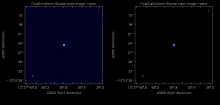
Stokes I.

Stokes Q.
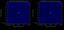
Stokes U.
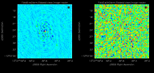
Stokes V.


Fig. 22. Comparison between images of the polarization calibrator without (left panels) and with (right panels) the D-term corrections applied.
Applying the calibrations and splitting of the corrected data

Now we will use applycal to apply the calibration tables that we generated in the previous sections. First, we apply the calibration tables to the polarization calibrator.
# In CASA
# Apply caltables to fields = 0
applycal(vis='3c286_Band6.ms',
         field='0',
         calwt=[True,True,False,False,False],
         gaintable=['3c286_Band6.ms.Bscan','3c286_Band6.ms.G2.polcal',
         '3c286_Band6.ms.Kcrs','3c286_Band6.ms.XY0','3c286_Band6.ms.Df0gen'],
         interp=['nearest','linear', 'linear','nearest', 'nearest'],
         gainfield=['', '','', '', ''],
         parang=True)
NEW: We first plot the complex plane again, and compare the results with Figure 17. Figure 23 shows clearly that the imaginary part is now zero, while the real part is corrected for the variation shown before; its corrected value is ~0.04.
Let's now examine the corrected amplitude and phase of the polarization calibrator.
# In CASA
plotms(vis='3c286_Band6.ms', xaxis='chan', yaxis='amp',
       ydatacolumn='corrected', selectdata=True, field='0',
       averagedata=True, avgchannel='',
       avgtime='1e9', avgscan=True,
       showgui=True,
       coloraxis='corr')


In Figure 24 we see that the XX,YY correlations have unitary amplitude, since we didn't scaled the flux. The XY,YX amplitude value is of the order of 0.04, which means the Stokes U of this source is ~0.04. This value is consistent with what the previous steps revealed. After the calibration all the phases are zero (Figure 25). To more clearly show the effect of the D-terms application on the polarization calibrator we also plot the corrected phases of the baseline DA48&DV23 (Figure 26). Comparing this result with Figure 16 we see that the XY and YX phases are now corrected and around zero.
We now apply the solutions from the phase calibrator (field='3') to the science target (field='4'). Its flux scale has also been bootstrapped to that of the flux calibrator, so it can serve as an amplitude and phase calibrator. We apply to these sources the polarization calibrations (Kcrs, XY0, and Df0gen) that we obtained for the polarization calibrator (field='0').
# In CASA
# Apply caltables to fields = 3 & 4
applycal(vis='3c286_Band6.ms',
         field='3,4',
         calwt=[True,True,False,False,False,False],
         gaintable = ['3c286_Band6.ms.Bscan','3c286_Band6.ms.G2ph','3c286_Band6.ms.flux',
         '3c286_Band6.ms.Kcrs','3c286_Band6.ms.XY0','3c286_Band6.ms.Df0gen'],
         interp=['nearest','linear','linear','nearest','nearest','nearest'],
         gainfield=['', '3', '3','', '', ''],
         parang=True)
- gaintable=['*.Bscan', '*.G2ph', '*.flux', '*.Kcrs', '*.XY0', '*.Df0gen']: these are all the tables to be applied to the data.
- interp=['nearest', 'linear', 'linear', 'nearest', 'nearest', 'nearest']: the corresponding interpolation method
- gainfield=[, '3', '3',, , ]: select the field from the corresponding gaintable. Here the phase calibrator gains are applied to both the calibrator itself and the target.
- parang=True: apply the parallactic angle correction
To check the effects of calibration on the scientific target we can compare the plot of imaginary vs real part before the calibration (xdatacolumn & ydatacolumn='data') and after (xdatacolumn & ydatacolumn='corrected'):
# In CASA
plotms(vis='3c286_Band6.ms', field='4',
        xaxis='real', yaxis='imag', spw='0',
	ydatacolumn='data', xdatacolumn='data', selectdata=True,
	averagedata=True, avgchannel='1000',
        avgtime='1e9', avgscan=True, plotrange=[-0.015,0.015,-0.015,0.015],
        coloraxis='corr',showgui=True)


You can see in these plots how the calibration has corrected the real and imaginary parts of the target visibilities. The imaginary parts of both the parallel and the cross-hands are close to zero, while the real parts are ~340 mJy and ~60 mJy, respectively.
We now split the scientific target (field 4) corrected data:
# In CASA
os.system('rm -rf 3c286_Band6.pol.cal.ms')
split(vis='3c286_Band6.ms',
      outputvis='3c286_Band6.pol.cal.ms',
      field='4',
      datacolumn='corrected',
      width='8')
Using the parameter width we average the channels, in order to reduce the size of the output file (3c286_Band6.pol.cal.ms will have 16 channels). In Band 3 TDM observations, averaging more than about 8 channels in full Stokes would produce significant bandwidth smearing.
Now you can continue on to the imaging guide.
References
- Synthesis Imaging in Radio Astronomy II, 1999, ASP Conference Series, Vol. 180, Editors: Taylor, G. B.; Carilli, C. L.; Perley, R. A.
- Interferometry and Synthesis in Radio Astronomy, 2nd Edition, 2001, Thompson, A.R., Moran, J.M., Swenson, G. W., Ed. Wiley
- AT polarization calibration, 1991, Sault, R. J., Killeen,N.E.B., & Kesteven, M.J., ATNF memo
- Understanding radio polarimetry. I. Mathematical foundations., 1996, Hamaker, J. P.; Bregman, J. D.; Sault, R. J., Astronomy and Astrophysics Supplement, v.117
Last checked on CASA Version 5.7.0.